Data and statistics
UAT 315 Artificial Intelligence, Data Analytics and Computer Vision for Unmanned Aircraft Systems
Lesson
By the end of this module you will be able to
- Compare data from RGB, thermal, multispectral and LiDAR sensors and the limits of each
- Explain that an image is an array of numbers, and compute NDVI from red and near-infrared bands
- Build features from raw data and scale them before feeding a model
- Describe the data cycle of an AI project from collection to post-deployment monitoring
Why this matters
The best artificial intelligence (AI) can do no better than the data it is given. One drone may carry several cameras, each measuring a different quantity. Without knowing what the values in a file mean, a developer might train a model to “read temperature” from a colour image that holds no measurement at all. This course starts with data, because most real-world AI work spends more time preparing data than choosing models.
The basic statistics used in this course were covered in UAT 106. Code examples here use synthetic data generated in the code, for learning only.
The main sensors on a drone
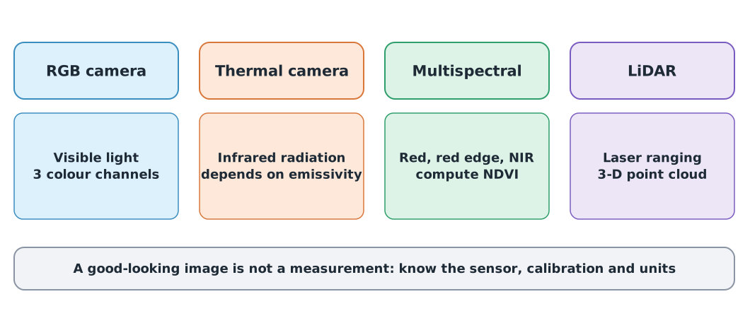
| Sensor | What it measures | Good for | Key limits |
|---|---|---|---|
| RGB camera | Red, green and blue light | Object detection, mapping | Depends on light and shadow; cannot see what is hidden |
| Thermal camera | Thermal infrared radiation | Finding people, inspecting solar panels | Temperature depends on emissivity; needs a radiometric camera |
| Multispectral camera | Reflectance in several bands, e.g. red, red edge, NIR | Crop health | Needs reflectance calibration |
| LiDAR | Range from laser pulses | Height models, under tree canopy | Large data, expensive equipment |
Emissivity is how efficiently a surface radiates heat. Teledyne FLIR explains that surfaces with emissivity below 0.5, such as polished metal, usually cannot be measured accurately, because the camera also sees heat reflected from other objects. A thermal image shown in colour is therefore not always a temperature reading; you need to know whether the camera records measurements (radiometric), as the drone knowledge hub’s unit on the limits of RGB and thermal images warns.
LiDAR data is usually stored as LAS files. The USGS specification for national mapping requires LAS version 1.4. Each point stores x, y and z coordinates, return intensity and return number.
An image is an array of numbers
A computer sees an image as an array of pixels. A 120 × 160 colour image holds 120 × 160 × 3 = 57,600 numbers, usually 8-bit integers from 0 to 255. Libraries may order channels differently: OpenCV uses BGR, not RGB. Pass the wrong order and the model sees wrong colours throughout.
A multispectral camera gives one image per band. NDVI (Normalized Difference Vegetation Index), proposed by Rouse and colleagues in 1974, uses the fact that healthy leaves reflect near-infrared (NIR) strongly but absorb red light. Its values run from −1 to +1.
import numpy as np

surfaces = {"healthy crop": (0.50, 0.08), "stressed crop": (0.30, 0.12), "bare soil": (0.25, 0.20), "water": (0.02, 0.05)}
for name, (nir, red) in surfaces.items():
    print(f"{name:<14} NIR {nir:.2f}  Red {red:.2f}  NDVI {(nir - red) / (nir + red):+.3f}")
healthy crop NIR 0.50 Red 0.08 NDVI +0.724
stressed crop NIR 0.30 Red 0.12 NDVI +0.429
bare soil NIR 0.25 Red 0.20 NDVI +0.111
water NIR 0.02 Red 0.05 NDVI -0.429These reflectances are made-up practice values. Healthy crops score high, stressed crops lower, bare soil near zero and water negative. Next, compute every pixel at once with numpy.
nir = np.array([[0.50, 0.48, 0.30, 0.25],
                [0.52, 0.45, 0.28, 0.24],
                [0.02, 0.03, 0.26, 0.00],
                [0.02, 0.02, 0.27, 0.00]])
red = np.array([[0.08, 0.09, 0.12, 0.20],
                [0.07, 0.10, 0.13, 0.21],
                [0.05, 0.05, 0.19, 0.00],
                [0.06, 0.05, 0.20, 0.00]])
total = nir + red
ndvi = np.divide(nir - red, total, out=np.full_like(total, np.nan), where=total > 0)
print(np.round(ndvi, 2))
print("vegetation pixels (NDVI > 0.5):", int(np.sum(ndvi > 0.5)), "  no-data pixels:", int(np.isnan(ndvi).sum()))
[[ 0.72 0.68 0.43 0.11]
[ 0.76 0.64 0.37 0.07]
[-0.43 -0.25 0.16 nan]
[-0.5 -0.43 0.15 nan]]
vegetation pixels (NDVI > 0.5): 4 no-data pixels: 2The two bottom-right pixels are zero in both bands, for example outside the image. Dividing directly gives an undefined value, so np.divide(..., where=...) puts nan in those pixels and reports them separately, rather than letting them become zero and be mistaken for soil.
Example 1 Building heights from LiDAR
A LiDAR point cloud gives the height z of every point. Height above ground is z minus the ground height. This example estimates the ground simply as the 5th percentile of all points, which only works for a small flat area.
rng = np.random.default_rng(345)
ground = rng.normal(12.0, 0.05, 900)
roof = rng.normal(18.5, 0.08, 80)
tree = rng.uniform(13.0, 21.0, 120)
z = np.concatenate([ground, roof, tree])
z_ground = np.percentile(z, 5)
height = z - z_ground
print(f"points {z.size}   estimated ground {z_ground:.2f} m")
print(f"points above 2 m: {int(np.sum(height > 2))}   highest {height.max():.1f} m above ground")
points 1100 estimated ground 11.92 m
points above 2 m: 182 highest 9.1 m above groundReal work uses far more sophisticated ground-classification algorithms, because real terrain slopes.
Features and scaling
A feature is a number given to a model. Raw flight-log data must first become meaningful features, such as the RMS vibration over one second or the mean current while hovering. Features have very different units and sizes: vibration may be around 0.1 g while current is around 20 A. Many models that rely on distances or gradients give too much weight to large numbers, so we standardise each feature to mean 0 and standard deviation 1.
from sklearn.preprocessing import StandardScaler

features = np.array([[0.11, 17.5], [0.13, 18.2], [0.21, 21.0], [0.12, 18.9], [0.18, 20.4]])
scaler = StandardScaler().fit(features)
print("mean", scaler.mean_.round(3), "  sd", scaler.scale_.round(3))
print(scaler.transform(features).round(2))
mean [ 0.15 19.2 ] sd [0.038 1.316]
[[-1.04 -1.29]
[-0.52 -0.76]
[ 1.56 1.37]
[-0.78 -0.23]
[ 0.78 0.91]]StandardScaler computes the standard deviation dividing by (not as in UAT 106), which suits scaling. The mean and standard deviation used for scaling must come from the training set only and then be applied to the test set. Computing them from all the data leaks test information into training without anyone noticing, which module 4 covers in detail.
The data cycle of an AI project
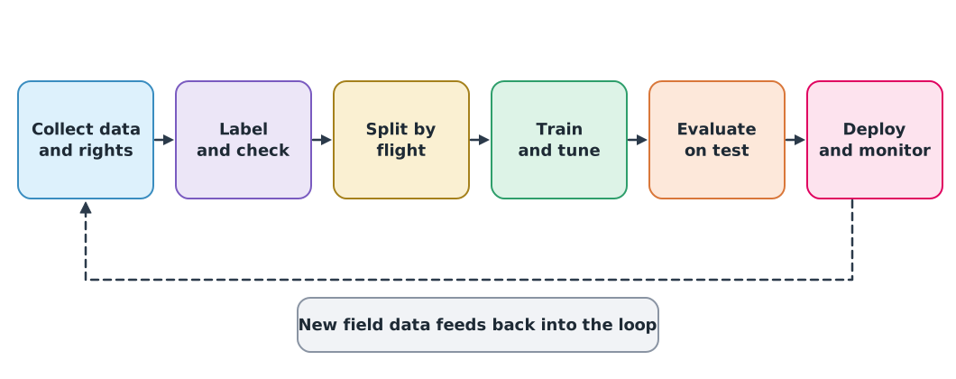
AI work does not end when training finishes. After deployment you must watch whether results stay good, because real conditions change: seasons change crop colour, or the camera model changes. New data that differs from training data is called data drift. Every step must record the source and usage rights of the data, as covered in UAT 313 and UAT 105.
Class activity
Activity: designing data for a mission
- In groups, choose a mission, such as finding a missing person in a forest, inspecting solar panels or assessing rice fields, and choose suitable sensors with reasons and limits.
- List the features you would use, with units and how each is computed from raw data.
- Read the knowledge unit on the limits of RGB and thermal images, and write three questions to ask a sender before trusting temperatures in a thermal image.
- Draw the data cycle for your mission, naming who is responsible and where quality checks happen at each step.
Common mistakes
Watch out
- Reading temperature from image colour with no measurement or scale
- Swapping channel order between RGB and BGR libraries
- Letting division by zero become a normal value instead of marking it as no data
- Scaling with all the data, leaking test data
- Thinking AI work ends at training, without monitoring for drift
Summary
- Each sensor measures a different quantity; reading temperature from a thermal image needs known emissivity and a radiometric camera
- An image is an array of numbers; NDVI comes from NIR and red, and no-data pixels must be handled explicitly
- Features must be meaningful and scaled with statistics from the training set only
- AI work is a cycle that needs post-deployment monitoring and a record of data rights at every step
Check your understanding
- What is NDVI for NIR = 0.40 and Red = 0.10?
- How many numbers are in a 100 × 200 pixel colour image?
- Why can a thermal camera not measure the temperature of polished metal accurately?
- A feature has mean 20 and standard deviation 2. What is 23 after standardisation?
- A LiDAR point is at 31.4 m and the ground at 12.0 m. How high is the point above the ground?
Answers
- numbers
- Polished metal has low emissivity, so the camera sees a lot of heat reflected from other objects
- m
Key formulas
| Normalized Difference Vegetation Index | |
| Standardisation | |
| Height above ground from LiDAR |
Key references
- Szeliski, R. (2022). Computer vision: Algorithms and applications (2nd ed.). Springer. link
- Géron, A. (2025). Hands-on machine learning with Scikit-Learn and PyTorch. O'Reilly. link
- U.S. Geological Survey. Landsat normalized difference vegetation index. link
- Rouse, J. W., Haas, R. H., Schell, J. A., & Deering, D. W. (1974). Monitoring vegetation systems in the Great Plains with ERTS. Third ERTS-1 Symposium, NASA. link
- Teledyne FLIR. How does emissivity affect thermal imaging? link
- U.S. Geological Survey. Lidar base specification: Update of LAS reference to R15 (LAS 1.4). link
- scikit-learn developers. Metrics and scoring: Quantifying the quality of predictions (scikit-learn 1.9). link
- OpenCV. OpenCV documentation. link
Further reading
Study the assigned knowledge units in advance, review media and take the module quiz
Descriptive statistics and probability distributions
Data handling and visualisation with Python
Limitations of RGB and thermal imagery
In class / field
Lecture, case discussion and in-class problem solving
Learning evidence: Quiz results and submitted exercises