Experiments and interpreting test results
UAT 106 Statistics and Data Analytics for Technology
Lesson
By the end of this module you will be able to
- Separate requirement, acceptance criterion, procedure and evidence, and order UAV test stages
- Design experiments using randomisation, replication and blocking
- Analyse a 2² factorial experiment for main effects and interaction
- Evaluate Type A and Type B measurement uncertainty, and report pass rates with confidence intervals
Why this matters
Good data comes not from clever analysis but from good experimental design before anyone flies. Fly all of brand A in the cool morning and all of brand B in the hot afternoon, and the measured difference may be the temperature, not the brand, and no analysis can separate them. This module brings the whole course together into a testing process that others can check.
From requirement to evidence
The drone knowledge hub’s unit on UAV testing and evidence analysis separates four things.
| What to write | Example |
|---|---|
| Requirement | Endurance no less than 20 minutes with a 1.0 kg payload at 25–35 °C |
| Acceptance criterion | The one-sided 95% lower bound of the mean exceeds 20 minutes, from at least 8 flights |
| Procedure | Start timing when the skids leave the ground, stop when the battery reaches 20%, hover at 10 m |
| Evidence | Every flight log, the results table, the analysis code and the weather |
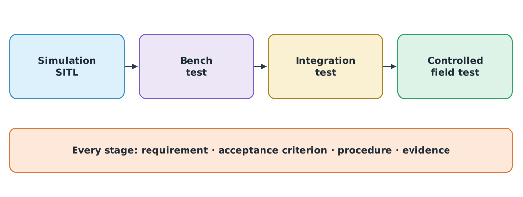
Write the acceptance criterion before seeing results. Testing moves from low risk to high risk, with each stage answering a different question; simulation results are not evidence about the real aircraft.
Principles of experimental design
Box, Hunter and Hunter’s Statistics for Experimenters stresses three principles:
- Randomisation: randomise the run order so factors that change over time, such as temperature or pilot skill, do not mix with the factor being studied
- Replication: repeat each condition several times with independent units to estimate variability
- Blocking: if testing spans several days, run every condition each day and account for the day in the analysis
import numpy as np

plan = [(payload, prop) for payload in (0.5, 1.0) for prop in ("standard", "efficient") for _ in range(3)]
rng = np.random.default_rng(2026)
order = rng.permutation(len(plan))
for run, idx in enumerate(order[:5], start=1):
    print(run, plan[idx])
print("...", len(plan), "runs in total")
1 (1.0, 'standard')
2 (0.5, 'standard')
3 (1.0, 'efficient')
4 (1.0, 'standard')
5 (1.0, 'efficient')
... 12 runs in totalThe 2² factorial experiment
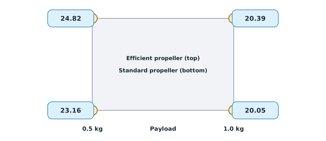
Changing one factor at a time misses something important: factors can act together. A factorial experiment tests every combination of factor levels at once. Here there are two factors with two levels each, payload 0.5 or 1.0 kg and a standard or efficient propeller, with three repeats per corner, 12 flights in all. The data is in factorial.csv.
import pandas as pd

fx = pd.read_csv("factorial.csv")
cell = fx.groupby(["payload_kg", "propeller"])["endurance_min"].mean()
print(cell.round(3).to_string())

light_std, light_eff = cell[(0.5, "standard")], cell[(0.5, "efficient")]
heavy_std, heavy_eff = cell[(1.0, "standard")], cell[(1.0, "efficient")]
payload_effect = (heavy_std + heavy_eff) / 2 - (light_std + light_eff) / 2
prop_effect = (light_eff + heavy_eff) / 2 - (light_std + heavy_std) / 2
interaction = ((heavy_eff - heavy_std) - (light_eff - light_std)) / 2
print(f"payload effect {payload_effect:+.2f} min   propeller effect {prop_effect:+.2f} min   interaction {interaction:+.2f} min")
payload_kg propeller
0.5 efficient 24.817
standard 23.160
1.0 efficient 20.393
standard 20.053
payload effect -3.76 min propeller effect +1.00 min interaction -0.66 minThe main effect of payload is a drop of about 3.8 minutes going from 0.5 to 1.0 kg, and the efficient propeller adds about 1 minute on average. But the negative interaction says the efficient propeller helps a lot with a light payload (1.66 minutes) and little with a heavy one (0.34 minutes). Testing the propeller at 0.5 kg alone would overstate its benefit for heavy delivery missions. These differences still need comparing with the spread between repeats before calling them significant.
Measurement uncertainty
Every measurement is uncertain. The GUM (JCGM 100:2008) describes two ways to evaluate uncertainty:
- Type A: statistical analysis of repeated observations, such as the standard error of a mean
- Type B: any other means, such as instrument resolution or a calibration certificate. If an instrument reads to 0.1 s, the true value is equally likely anywhere within ±0.05 s of the reading, so a rectangular distribution gives
Example 1 Uncertainty of a hover time
Five testers time the same hover with stopwatches reading to 0.1 s.
import math
import statistics

readings = [1212.4, 1212.9, 1212.1, 1212.6, 1212.5]
mean = statistics.mean(readings)
u_a = statistics.stdev(readings) / math.sqrt(len(readings))
u_b = 0.05 / math.sqrt(3)
u_c = math.sqrt(u_a ** 2 + u_b ** 2)
print(f"mean {mean:.2f} s   u_A {u_a:.3f} s   u_B {u_b:.3f} s   u_c {u_c:.3f} s")
print(f"result {mean:.2f} s ± {2 * u_c:.2f} s (k = 2)")
mean 1212.50 s u_A 0.130 s u_B 0.029 s u_c 0.134 s
result 1212.50 s ± 0.27 s (k = 2)The uncertainty from human timing (Type A) is much larger than the stopwatch resolution (Type B), so a finer stopwatch would barely help; the method must change, for example by taking times from the flight controller log. When reporting expanded uncertainty under the GUM, always state the coverage factor ; this example uses .
Reporting pass rates within their limits
The drone knowledge hub’s unit on exercises and evaluating simulated missions warns that pass criteria must be defined before testing, and runs that did not finish must be reported separately, never deleted. A pass rate from a limited number of trials is uncertain too.
from scipy import stats

passed, total = 80, 100
ci = stats.binomtest(passed, total).proportion_ci(confidence_level=0.95)
print(f"pass rate {passed / total:.0%}   95% CI (Clopper-Pearson) [{ci.low:.3f}, {ci.high:.3f}]")
ci_small = stats.binomtest(8, 10).proportion_ci(confidence_level=0.95)
print(f"8 of 10 runs: 95% CI [{ci_small.low:.3f}, {ci_small.high:.3f}]")
pass rate 80% 95% CI (Clopper-Pearson) [0.708, 0.873]
8 of 10 runs: 95% CI [0.444, 0.975]An 80% pass rate from 100 runs has a confidence interval of about 71% to 87%, but 8 out of 10 runs gives about 44% to 97%. The same 80% means very different things. And the pass rate applies only to the model and conditions tested, not to the chance of success in the field.
What a good test report contains
Test ID and requirement, the acceptance criterion written before testing, environment, settings and firmware version, raw data with units, analysis method and assumptions, sample size, confidence intervals and uncertainty, excluded data with reasons, and conclusions that go no further than the data.
Module lab
Lab: designing and analysing a propeller test
- Write a test plan using the table in this lesson (requirement, acceptance criterion, procedure, evidence) for comparing two propellers, and have a classmate review it before opening the data.
- Analyse
factorial.csvfor main effects, interaction and the standard deviation between repeats at each corner, and judge which effects clearly exceed the repeat-to-repeat variation. - Draw an interaction plot (payload on the horizontal axis, one line per propeller) and explain what non-parallel lines mean.
- Evaluate both Type A and Type B uncertainty for endurance timing in your own test, and write a complete one-page test report.
Common mistakes
Watch out
- Setting the acceptance criterion after seeing results
- Not randomising the run order, so time-varying factors mix with the factor studied
- Changing one factor at a time, which hides interactions
- Reporting a measurement without uncertainty, or without stating
- Silently removing failed runs, or reporting a pass rate without the number of runs
Summary
- Separate requirement, acceptance criterion, procedure and evidence; write criteria before seeing results; test from low to high risk
- Randomisation, replication and blocking make experimental results trustworthy
- Factorial experiments reveal both main effects and interactions, which one-factor-at-a-time testing cannot
- Report both Type A and Type B uncertainty, and give pass rates with the number of runs and a confidence interval
Check your understanding
- Why randomise the flight order when testing two battery brands?
- The four corner means are A−B− = 20, A+B− = 24, A−B+ = 22, A+B+ = 30. What is the main effect of A?
- From question 2, what is the AB interaction?
- A scale reads to 0.01 kg. What is the Type B uncertainty from its resolution?
- A system passes 20 of 20 runs. Can we conclude that “it always passes, 100%”?
Answers
- So that time-varying factors, such as temperature or pilot skill, do not mix with the brand effect
- kg, so kg
- No: the 95% confidence interval of the pass rate still has a lower bound of about 83%, and the result holds only for the conditions tested
Key formulas
| Main effect of factor A in a 2² factorial | |
| AB interaction | |
| Type B uncertainty from a rectangular distribution | |
| Combined and expanded uncertainty |
Key references
- Box, G. E. P., Hunter, J. S., & Hunter, W. G. (2005). Statistics for experimenters: Design, innovation, and discovery (2nd ed.). Wiley. link
- Montgomery, D. C., & Runger, G. C. (2018). Applied statistics and probability for engineers (7th ed.). Wiley. link
- JCGM. (2008). Evaluation of measurement data — Guide to the expression of uncertainty in measurement (JCGM 100:2008). BIPM. link
- JCGM. (2012). International vocabulary of metrology — Basic and general concepts and associated terms (VIM, JCGM 200:2012). BIPM. link
- NIST/SEMATECH. e-Handbook of statistical methods. National Institute of Standards and Technology. link
- The SciPy community. Statistical functions (scipy.stats), SciPy 1.18 documentation. link
- Wasserstein, R. L., & Lazar, N. A. (2016). The ASA statement on p-values: Context, process, and purpose. The American Statistician, 70(2), 129–133. link
Further reading
Study the assigned knowledge units in advance, review media and take the module quiz
UAV testing and evidence analysis
Interpreting endurance test results
Exercises and evaluation of simulated missions
In class / field
Lab or field practice from worksheets with a safety checklist
Learning evidence: Checked worksheets and quiz results