Control systems and models
UAT 206 Fundamentals of Control and Autopilot Systems
Lesson
By the end of this module you will be able to
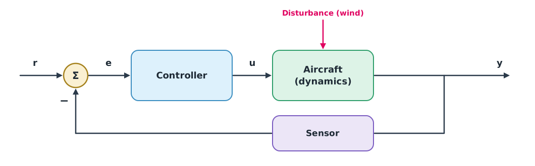
- Explain the parts of a closed-loop control system with a block diagram
- Build a first-order motor model and find its time constant from step-response data
- Write the vertical dynamics of a multicopter and linearise them around hover
- Read first-order and second-order transfer functions
Why this matters
A flight controller decides hundreds of times per second how hard to drive each motor. Without understanding how the drone responds to commands, tuning becomes guesswork. UAT 314 covered feedback and PID; this course goes deeper into models, response, practical PID implementation and the structure of the PX4 and ArduPilot autopilots.
The whole course uses one hypothetical case: a lab tuning a 1.5 kg training quadcopter in SITL before real flights. All numbers are made up for practice. The Python code for every module can be downloaded from /downloads/uat-206/.
The closed-loop block diagram
A closed-loop system measures the output and compares it with the desired value to get the error . The controller uses to compute a command for the aircraft, which is also pushed by disturbances such as wind. A sensor measures the result and feeds it back for the next comparison, like a driver watching the road and correcting the steering all the time (Åström and Murray, 2021).
A first-order motor model
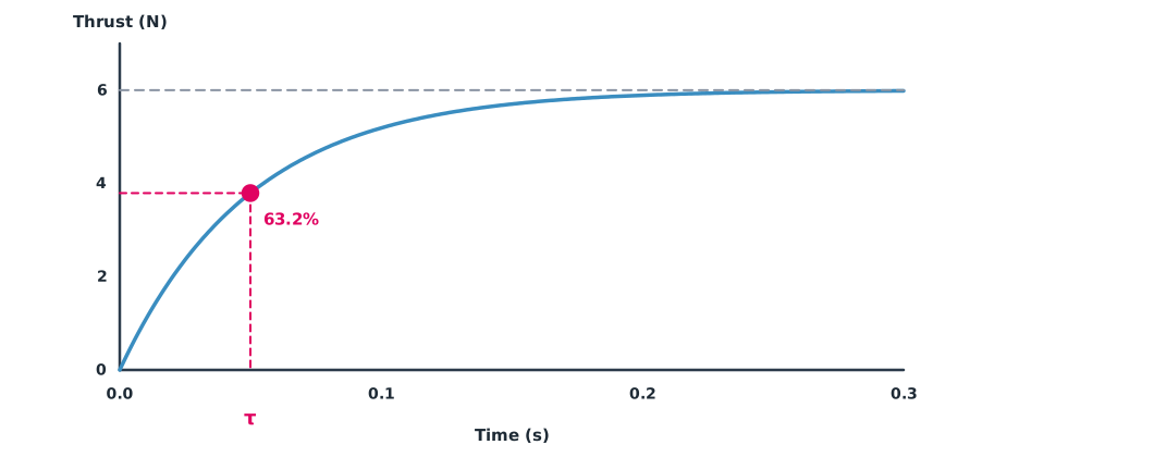
When the throttle steps up, the propeller does not speed up instantly because of its inertia. Thrust rises as a first-order response , where is the time constant, the time for the response to reach 63.2% of its final value. As a transfer function, a way of writing the input–output relationship in the Laplace domain, it is (Nise, 2019).
Example 1 Finding a motor’s time constant on a test stand
The throttle is stepped and a load cell records thrust every 10 ms.
import math

DT = 0.01
thrust = [0.0, 1.09, 1.98, 2.71, 3.3, 3.79, 4.19, 4.52, 4.79, 5.01, 5.19, 5.34, 5.46, 5.55, 5.64,
          5.7, 5.76, 5.8, 5.84, 5.87, 5.89, 5.91, 5.93, 5.94, 5.95, 5.96, 5.97, 5.97, 5.98, 5.98, 5.99]
final = thrust[-1]
target = 0.632 * final
i = next(k for k, v in enumerate(thrust) if v >= target)
t63 = (i - 1) * DT + (target - thrust[i - 1]) / (thrust[i] - thrust[i - 1]) * DT
print(f"final thrust {final:.2f} N, 63.2% = {target:.2f} N, tau from the curve = {t63 * 1000:.1f} ms")

pts = [(k * DT, math.log(1 - v / final)) for k, v in enumerate(thrust[:15])]
slope = sum(t * y for t, y in pts) / sum(t * t for t, _ in pts)
print(f"tau from a log fit of the first 0.14 s = {-1 / slope * 1000:.1f} ms")
final thrust 5.99 N, 63.2% = 3.79 N, tau from the curve = 49.9 ms
tau from a log fit of the first 0.14 s = 49.6 msThe two methods agree at about 50 ms. Reading the 63.2% point is simple but uses only a few samples; fitting a line uses the whole range, so it tolerates noise better. This value tells us the rate controller should not demand changes faster than the motors can follow.
Vertical dynamics and linearisation
Vertically, the total thrust works against the weight , giving . Propeller thrust is roughly proportional to the square of throttle, , which is nonlinear. But we mostly control around hover, so a straight line around that point is a good approximation: . Beard and McLain (2012) use the same approach for small unmanned aircraft.
Example 2 Hover throttle and local gain
A 1.5 kg drone with four motors, each giving 8 N maximum thrust at full throttle (hypothetical values).
import math

M, G, N_MOTORS, K_MAX = 1.5, 9.80665, 4, 8.0      # kg, m/s², number of motors, N at full throttle
t_hover = M * G / N_MOTORS
u_hover = math.sqrt(t_hover / K_MAX)
gain = N_MOTORS * 2 * K_MAX * u_hover                # N per 1.0 throttle (all motors together)
print(f"hover thrust per motor {t_hover:.2f} N, hover throttle {u_hover:.3f}")
print(f"local gain {gain:.1f} N per unit throttle -> +0.01 throttle gives {gain * 0.01 / M:.2f} m/s^2")
print(f"thrust-to-weight ratio {N_MOTORS * K_MAX / (M * G):.2f}")
hover thrust per motor 3.68 N, hover throttle 0.678
local gain 43.4 N per unit throttle -> +0.01 throttle gives 0.29 m/s^2
thrust-to-weight ratio 2.18A hover throttle of about 0.68 leaves limited room to climb. Adding payload raises hover throttle and changes the local gain, so tuned gains may no longer fit; the hover throttle must be re-checked whenever the weight or battery changes.
Second-order transfer functions
Many systems combine two first-order parts, or have mass and spring behaviour, so they respond as second-order systems. The standard form is , where is the natural frequency and is the damping ratio, which sets how much the response oscillates. Module 2 uses this form to study response and stability.
Module lab
Lab: motor test stand
- Mount a motor and propeller on a thrust stand with a propeller guard, following the lab’s safety rules.
- Command several throttle levels, record steady thrust and find in .
- Step the throttle, record thrust against time and use the code from Example 1 to find .
- Use the code from Example 2 with the measured values to find hover throttle with and without payload.
- Draw the block diagram of the altitude controller to be used in Module 3, stating the unit of every signal.
Common mistakes
Watch out
- Assuming motors respond instantly.
- Using the linear model far from hover.
- Forgetting that payload changes hover throttle.
- Mixing units in the block diagram.
- Testing motors without a propeller guard.
Summary
- A closed loop measures the output, compares it with the reference and keeps correcting, while disturbances act on it.
- A motor can be approximated by a first-order model; is the time to reach 63.2% of the final value.
- Vertical dynamics with thrust are linearised around hover.
- A second-order system is defined by and .
Check your understanding
- A first-order system has s. When does the response reach 63.2% of its final value?
- At , what percentage of the final value has been reached?
- A 2 kg drone has four motors. What is the hover thrust per motor?
- If and hover thrust per motor is 2 N, what is the hover throttle?
- Why linearise the model around hover?
Answers
- At 0.1 s.
- N
- Most controller design tools work for linear systems, and the drone operates mostly around hover.
Key formulas
| First-order model | |
| Vertical dynamics | |
| Motor thrust and linearisation |
Key references
- Nise, N. S. (2019). Control systems engineering (8th ed.). Wiley. link
- Åström, K. J., & Murray, R. M. (2021). Feedback systems: An introduction for scientists and engineers (2nd ed.). Princeton University Press. link
- Ogata, K. (2010). Modern control engineering (5th ed.). Pearson.
- Beard, R. W., & McLain, T. W. (2012). Small unmanned aircraft: Theory and practice. Princeton University Press. link
Further reading
Study the assigned knowledge units in advance, review media and take the module quiz
In class / field
Lab or field practice from worksheets with a safety checklist
Learning evidence: Checked worksheets and quiz results