Module 2/5 · Weeks 4–6 · 27 h

Response and stability

UAT 206 Fundamentals of Control and Autopilot Systems

About 90 minDraft, awaiting reviewLast updated 28 September 2026

By the end of this module you will be able to

Explain step-response metrics such as rise time, overshoot and settling time
Compute the overshoot and settling time of a second-order system from its damping ratio and natural frequency
Explain stability from pole locations in the s-plane
Compute the effect of time delay on phase margin and find the critical delay

Prerequisites: UAT 206 Module 1

Why this matters

When tuning a drone, we check whether a step tilt command is followed quickly, whether it overshoots and how soon it settles. These quantities have names and formulas tied to the model. Knowing them tells us which way to adjust the gains, and what makes a system unstable, oscillating until it can no longer be controlled.

Step-response metrics

Åström and Murray (2021) define the main metrics as:

Rise time ( $T_{r}$ ): the time for the response to go from 10% to 90% of its final value.
Overshoot ( $M_{p}$ ): the maximum amount above the final value, as a fraction.
Settling time ( $T_{s}$ ): the time after which the response stays within ±2% of its final value.

For the standard second-order system, $M_{p} = e^{- π ζ / 1 - ζ^{2}}$ and $T_{s} \approx 4/ (ζ ω_{0})$ . The book notes that $ζ = 0.5$ gives 16% overshoot and $ζ = 1/ 2$ gives 4%.

Graph of step response against time from 0 to 3 seconds with four curves. Zeta 0.3 in pink overshoots to about 1.37 and oscillates. Zeta 0.5 in gold overshoots to about 1.16. Zeta 0.707 in blue overshoots slightly. Zeta 1.0 in green rises slowest without overshoot. A dashed horizontal line at 1 — Figure 1 Second-order step responses for several ζ

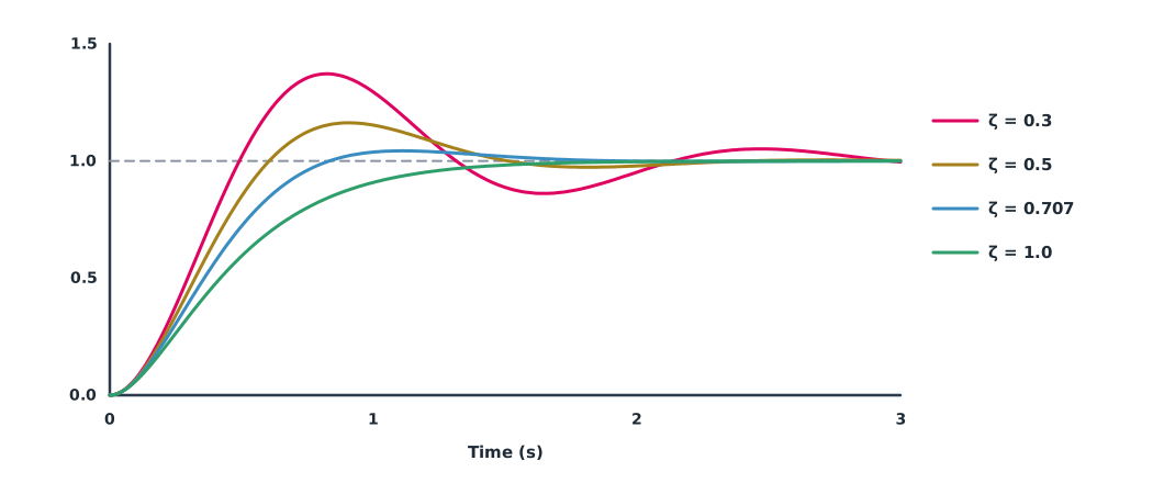
Example 1 Simulation versus formula

A second-order system with a natural frequency of 4 rad/s, simulated with 1 ms steps.

import math

W0, DT, T_END = 4.0, 0.001, 6.0

def simulate(zeta):
    y = v = 0.0
    out = []
    for _ in range(int(T_END / DT)):
        a = W0 ** 2 * (1 - y) - 2 * zeta * W0 * v
        v += a * DT
        y += v * DT
        out.append(y)
    return out

for zeta in (0.3, 0.5, 0.707, 1.0):
    ys = simulate(zeta)
    over = max(ys) - 1
    formula = math.exp(-math.pi * zeta / math.sqrt(1 - zeta ** 2)) if zeta < 1 else 0.0
    ts = next(i * DT for i in range(len(ys)) if all(abs(v - 1) <= 0.02 for v in ys[i:]))
    print(f"zeta {zeta:<5}: overshoot {max(over, 0):6.1%} (formula {formula:5.1%}), "
          f"settling {ts:.2f} s (4/(zeta*w0) = {4 / (zeta * W0):.2f} s)")

zeta 0.3  : overshoot  37.2% (formula 37.2%), settling 2.81 s (4/(zeta*w0) = 3.33 s)
zeta 0.5  : overshoot  16.3% (formula 16.3%), settling 2.02 s (4/(zeta*w0) = 2.00 s)
zeta 0.707: overshoot   4.3% (formula  4.3%), settling 1.49 s (4/(zeta*w0) = 1.41 s)
zeta 1.0  : overshoot   0.0% (formula  0.0%), settling 1.46 s (4/(zeta*w0) = 1.00 s)

Simulated overshoot matches the formula. The settling-time formula is an approximation, close for $ζ$ around 0.5–0.7 but clearly off at $ζ = 0.3$ and 1.0. Drones usually want $ζ$ around 0.6–0.8: a small overshoot with a fast response.

Stability and poles

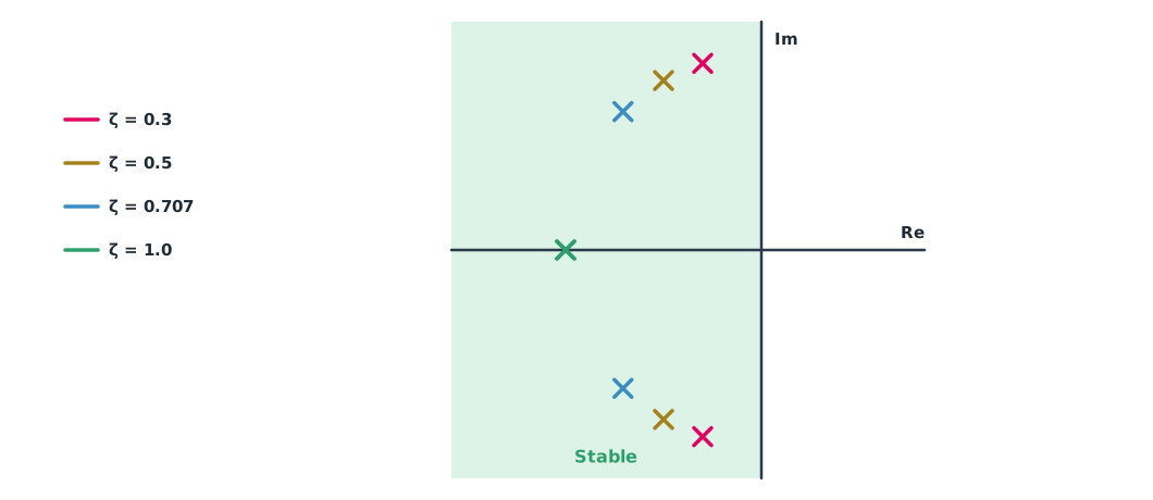
Poles are the roots of a transfer function’s denominator. A second-order system has poles at $- ζ ω_{0} \pm i ω_{0} 1 - ζ^{2}$ . A system is stable when every pole lies in the left half of the s-plane. Poles far from the imaginary axis respond and settle quickly, while poles with a large imaginary part relative to the real part oscillate a lot. If a pole crosses into the right half, the response grows without bound.

The s-plane with Re on the horizontal axis and Im on the vertical axis. The left half is shaded green and labelled stable. Four pairs of crosses: zeta 0.3 in pink near the vertical axis and high up, zeta 0.5 in gold, zeta 0.707 in blue at 45 degrees, zeta 1.0 in green as a double pole on the real axis. All pairs are the same distance from the origin — Figure 2 Pole locations in the s-plane

Time delay eats phase

Real systems have time delay from sensor filters, computation and motors. Åström and Murray show that a delay $τ_{d}$ does not change signal magnitude but adds phase lag $ω τ_{d}$ at frequency $ω$ , reducing the phase margin. The book suggests a reasonable phase margin of about 30–60°; at zero the system oscillates indefinitely.

Example 2 Delay in a rate loop

A simple rate-loop model $L (s) = K e^{- s τ_{d}} / s$ with $K = 20$ rad/s. The crossover frequency equals $K$ , so the phase margin is $90° - K τ_{d}$ (in degrees).

import math

K, DT = 20.0, 0.0005

def run(delay):
    n = int(round(delay / DT))
    buf = [0.0] * n
    y, out = 0.0, []
    for _ in range(int(3 / DT)):
        seen = buf[0] if n else y
        y += DT * K * (1 - seen)
        if n:
            buf = buf[1:] + [y]
        out.append(y)
    return out

print(f"critical delay (phase margin 0) = {math.pi / (2 * K) * 1000:.1f} ms")
for delay in (0.0, 0.02, 0.05, 0.075, 0.09):
    ys = run(delay)
    pm = 90 - K * delay * 180 / math.pi
    tail = max(abs(1 - v) for v in ys[-1000:])
    print(f"delay {delay * 1000:>4.0f} ms: phase margin {pm:5.1f} deg, peak {max(ys):6.2f}, "
          f"error in last 0.5 s {tail:.3f}")

critical delay (phase margin 0) = 78.5 ms
delay    0 ms: phase margin  90.0 deg, peak   1.00, error in last 0.5 s 0.000
delay   20 ms: phase margin  67.1 deg, peak   1.00, error in last 0.5 s 0.000
delay   50 ms: phase margin  32.7 deg, peak   1.50, error in last 0.5 s 0.000
delay   75 ms: phase margin   4.1 deg, peak   2.00, error in last 0.5 s 0.319
delay   90 ms: phase margin -13.1 deg, peak  25.51, error in last 0.5 s 24.513

A delay of only 50 ms makes a system that never overshot overshoot by half. Near 78.5 ms it oscillates without settling, and beyond that the oscillation grows without bound. This is why an overly delaying gyro filter can make a drone oscillate even though the PID gains are unchanged.

Module lab

Lab: response metrics and delay

Use the code from Example 1 with three values of $ω_{0}$ and see how overshoot and settling time change.
Plot the poles for each case on graph paper and compare with Figure 2.
Use the code from Example 2, change $K$ and find the new critical delay, comparing with $π / (2 K)$ .
In SITL, gradually add delay or lower the gyro filter frequency and watch the oscillation in the log.
Record your conclusion on the $ζ$ and phase margin to aim for on the lab drone.

Common mistakes

Watch out

Demanding zero overshoot, making the system too slow.
Always using the settling-time formula instead of measuring.
Ignoring delay from filters and computation.
Looking at one response only, missing a small continuous oscillation.
Changing several values at once, so the cause of a change is unclear.

Summary

The main metrics are $T_{r}$ (10–90%), $M_{p}$ and $T_{s}$ (±2%).
For second-order systems $M_{p} = e^{- π ζ / 1 - ζ^{2}}$ and $T_{s} \approx 4/ (ζ ω_{0})$ .
A system is stable when all poles are in the left half of the s-plane.
Time delay eats phase $ω τ_{d}$ , reducing phase margin until the system can oscillate.

Check your understanding

About what overshoot does $ζ = 0.5$ give?
With $ζ = 0.5$ and $ω_{0} = 8$ rad/s, what is the approximate settling time?
What do poles at $+ 1 \pm 2 i$ say about the system?
A loop with a 20 rad/s crossover has a 10 ms delay. How many degrees of phase are lost?
From question 4, if the original phase margin was 90°, what remains?

Answers

About 16%.
$4/ (0.5 \times 8) = 1$ s
It is unstable: the positive real part makes the oscillation grow.
$20 \times 0.01 = 0.2$ rad $\approx 11.5°$
About 78.5°.

Key formulas

Second-order overshoot	$M_{p} = e^{- π ζ / 1 - ζ^{2}}$
Settling time (2%)	$T_{s} \approx \frac{4}{ζ ω _{0}}$
Phase taken by a time delay	$∠ e^{- iω τ_{d}} = - ω τ_{d}$

Key references

Åström, K. J., & Murray, R. M. (2021). Feedback systems: An introduction for scientists and engineers (2nd ed.). Princeton University Press. link
Nise, N. S. (2019). Control systems engineering (8th ed.). Wiley. link
Ogata, K. (2010). Modern control engineering (5th ed.). Pearson.

In class / field

Lab or field practice from worksheets with a safety checklist

Learning evidence: Checked worksheets and quiz results

Module quiz

This is a formative self-check, not a graded exam

Knowledge domain: Control, autopilot and navigation · Mathematics, physics and statistics

Response and stability

By the end of this module you will be able to

Why this matters

Step-response metrics

Stability and poles

Time delay eats phase

Module lab

Common mistakes

Summary

Check your understanding

Key formulas

Key references

Further reading

Dynamic models and transfer functions

In class / field

Module quiz

Response and stability

Lesson

By the end of this module you will be able to

Why this matters

Step-response metrics

Stability and poles

Time delay eats phase

Module lab

Common mistakes

Summary

Check your understanding

Key formulas

Key references

Further reading

Dynamic models and transfer functions

In class / field

Module quiz