Computer vision
UAT 315 Artificial Intelligence, Data Analytics and Computer Vision for Unmanned Aircraft Systems
Lesson
By the end of this module you will be able to
- Explain convolution and use OpenCV to segment objects by colour, count them and find their boxes
- Explain the structure of a convolutional neural network (CNN) and its development from LeNet to ResNet
- Distinguish image classification, object detection and segmentation, and explain the detection pipeline including NMS
- Track an object with a simple Kalman filter and explain sensor fusion
Why this matters
A camera is the cheapest, most informative sensor on a drone. Computer vision lets drones find disaster victims, count trees, inspect cracks or follow objects. The methods range from classical image processing, where every step can be explained, to deep learning, which is more accurate but needs careful data and evaluation. Users must know what each method can do and where it fails.
Convolution and image processing
Convolution slides a small filter (kernel) across the image, multiplying and summing values at each position. Different filters give different effects, such as blurring or edge finding. A horizontal Sobel filter responds strongly where brightness changes from left to right.
import numpy as np

image = np.array([[10, 10, 10, 200, 200],
                  [10, 10, 10, 200, 200],
                  [10, 10, 10, 200, 200],
                  [10, 10, 10, 200, 200]], dtype=float)
sobel_x = np.array([[-1, 0, 1], [-2, 0, 2], [-1, 0, 1]], dtype=float)
out = np.zeros((image.shape[0] - 2, image.shape[1] - 2))
for i in range(out.shape[0]):
    for j in range(out.shape[1]):
        out[i, j] = np.sum(sobel_x * image[i:i + 3, j:j + 3])
print(out)
[[ 0. 760. 760.]
[ 0. 760. 760.]]The response is zero where brightness is constant and high at the boundary between 10 and 200, which is the object’s edge. In a CNN, filters like this are not designed by people; they are learned from data.
Example 1 Finding orange boxes on grass with OpenCV
Build a synthetic 120 × 160 image with a noisy green background and three orange boxes, then isolate orange in the HSV colour space (hue, saturation, value), which separates colours more easily than BGR.
import cv2

rng = np.random.default_rng(345)
frame = np.full((120, 160, 3), (60, 130, 70), np.uint8)
frame = np.clip(frame.astype(int) + rng.integers(-15, 16, frame.shape), 0, 255).astype(np.uint8)
truth = [(20, 30, 16, 12), (90, 70, 20, 14), (130, 20, 10, 10)]
for x, y, w, h in truth:
    frame[y:y + h, x:x + w] = (20, 120, 240)

hsv = cv2.cvtColor(frame, cv2.COLOR_BGR2HSV)
mask = cv2.inRange(hsv, (5, 150, 150), (25, 255, 255))
count, labels, stats, centroids = cv2.connectedComponentsWithStats(mask)
found = sorted(tuple(int(v) for v in s[:4]) for s in stats[1:])
print("objects found:", count - 1)
print("boxes (x, y, w, h):", found)
objects found: 3
boxes (x, y, w, h): [(20, 30, 16, 12), (90, 70, 20, 14), (130, 20, 10, 10)]This method is simple and fully explainable, but it only works when objects have a distinctive colour and the light is steady. Shadows, evening light or similarly coloured objects break the fixed colour range at once, which is why real systems use deep learning.
Convolutional neural networks
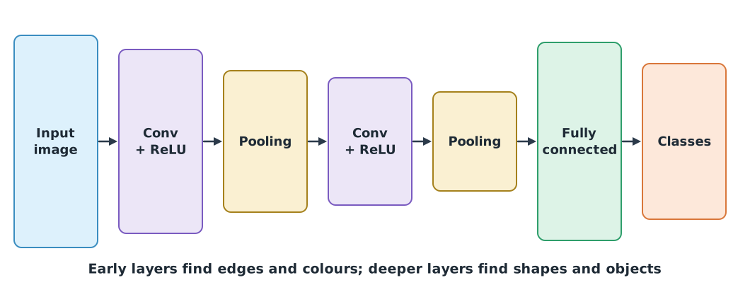
A CNN (convolutional neural network) stacks many convolution layers. Early layers learn edges and colours; deeper layers learn shapes and objects. Pooling layers shrink the data, and fully connected layers decide the class.
| Year | Work | Key point |
|---|---|---|
| 1998 | LeNet (LeCun et al.) | A CNN reading handwritten digits |
| 2012 | AlexNet (Krizhevsky et al.) | A deep CNN on GPUs won the ImageNet challenge by a wide margin |
| 2016 | ResNet (He et al.) | Skip (residual) connections made very deep networks trainable |
| 2016 | YOLO (Redmon et al.) | Detects objects in the whole image in one pass, fast enough for real time |
| 2023 | Segment Anything (Kirillov et al.) | A segmentation model that works on varied images without retraining |
Classify, detect and segment
- Image classification says what the whole image is, e.g. “contains flooding”
- Object detection says which objects are where, as rectangular boxes with confidence scores
- Segmentation gives a class for every pixel, e.g. water, road, building
The YOLO family is a popular detector on drones. Ultralytics’ newest release at the time of writing is YOLO26 (January 2026). It is licensed AGPL-3.0; closed-source products need a paid Enterprise licence, as the drone knowledge hub’s unit on computer vision and edge AI warns.
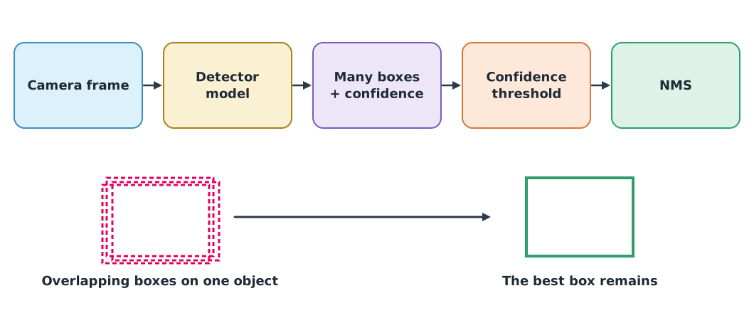
A detector often outputs several overlapping boxes on one object. NMS (non-maximum suppression) keeps the highest-scoring box and removes others that overlap it beyond a threshold. Overlap is measured with IoU: the intersection area divided by the union area.
def iou(a, b):
    ax, ay, aw, ah = a
    bx, by, bw, bh = b
    inter_w = max(0, min(ax + aw, bx + bw) - max(ax, bx))
    inter_h = max(0, min(ay + ah, by + bh) - max(ay, by))
    inter = inter_w * inter_h
    return inter / (aw * ah + bw * bh - inter)


def nms(boxes, scores, iou_threshold=0.5):
    order = sorted(range(len(boxes)), key=lambda i: scores[i], reverse=True)
    keep = []
    for i in order:
        if all(iou(boxes[i], boxes[k]) < iou_threshold for k in keep):
            keep.append(i)
    return keep


candidates = [(88, 69, 22, 15), (90, 70, 20, 14), (92, 72, 19, 13), (20, 30, 16, 12)]
scores = [0.81, 0.93, 0.66, 0.88]
print("IoU of box 0 and box 1:", round(iou(candidates[0], candidates[1]), 3))
print("kept after NMS:", [(candidates[i], scores[i]) for i in nms(candidates, scores)])
IoU of box 0 and box 1: 0.848
kept after NMS: [((90, 70, 20, 14), 0.93), ((20, 30, 16, 12), 0.88)]The first three boxes cover the same object; NMS keeps only the 0.93 box and keeps the box on the other object. The NMS IoU threshold must be chosen with care: set too low, two adjacent objects are cut down to one.
Tracking and data fusion
Frame-by-frame detection does not know whether a box in this frame and the last is the same object. Tracking links results across frames and uses a motion model to reduce noise. The Kalman filter, proposed by Kalman in 1960, blends predictions from a model with measurements, weighting each by its uncertainty. The same idea drives sensor fusion, such as combining GNSS with the IMU in a flight controller.
Example 2 Tracking a moving object
An object moves 2 m per frame, and positions measured from images have an error with standard deviation 1.5 m. Use a one-dimensional constant-velocity Kalman filter.
steps, speed, meas_sd = 30, 2.0, 1.5
truth_pos = speed * np.arange(steps)
measured = truth_pos + rng.normal(0, meas_sd, steps)

F = np.array([[1.0, 1.0], [0.0, 1.0]])
H = np.array([[1.0, 0.0]])
Q = np.diag([0.01, 0.01])
R = np.array([[meas_sd ** 2]])
x = np.array([measured[0], 0.0])
P = np.diag([R[0, 0], 4.0])
estimates = []
for z in measured:
    x = F @ x
    P = F @ P @ F.T + Q
    K = P @ H.T @ np.linalg.inv(H @ P @ H.T + R)
    x = x + (K @ (np.array([z]) - H @ x)).ravel()
    P = (np.eye(2) - K @ H) @ P
    estimates.append(x[0])
estimates = np.array(estimates)

rmse = lambda e: np.sqrt(np.mean(e ** 2))
print(f"RMSE of raw measurements (last 20 frames) {rmse(measured[10:] - truth_pos[10:]):.2f} m")
print(f"RMSE of Kalman estimates (last 20 frames) {rmse(estimates[10:] - truth_pos[10:]):.2f} m")
print(f"estimated speed {x[1]:.2f} m per frame")
RMSE of raw measurements (last 20 frames) 1.61 m
RMSE of Kalman estimates (last 20 frames) 0.68 m
estimated speed 1.97 m per frameAfter a few frames the filter gives positions far closer to the truth than the raw measurements, and it also estimates the speed, which was never measured. The filter has not settled in the first frames, so both are compared over the same last 20 frames.
Class activity
Activity: matching vision methods to tasks
- For three tasks, counting oil palms, assessing flooded area and finding victims at night, choose classification, detection or segmentation, and which camera to use.
- In Example 1, add a shadow by halving the brightness of one box, and see how colour segmentation fails. Discuss why a CNN can cope.
- Lower the NMS IoU threshold to 0.1 for boxes on two adjacent objects and explain the result.
- Read the knowledge unit on AI for screening disaster imagery and summarise why model output should be a list for checking, not a verdict.
Common mistakes
Watch out
- Using fixed colour ranges where the light changes
- Using image classification when you need the positions of several objects
- Setting the NMS threshold too low, so adjacent objects vanish
- Treating confidence as the probability of being right without checking on test data
- Not checking model and data licences before commercial use
Summary
- Convolution slides a filter over the image; classical processing is explainable but fragile under changing light
- CNNs learn their filters from data, evolving from LeNet to ResNet and detectors such as YOLO
- Classification, detection and segmentation answer different questions; detectors need a confidence threshold and NMS
- The Kalman filter blends predictions and measurements for tracking and sensor fusion
Check your understanding
- “Label every pixel as water or not” is which kind of task?
- Two boxes of 50 px² each overlap by 25 px². What is their IoU?
- Why segment colours in HSV rather than BGR?
- What does NMS do?
- When does a Kalman filter give more weight to the measurement?
Answers
- Semantic segmentation
- The union is , so IoU
- HSV separates colour (hue) from brightness, so colour ranges are easier to set and more robust to brightness changes
- It removes overlapping boxes on one object, keeping the highest-scoring box
- When the measurement uncertainty is small compared with the prediction uncertainty, making close to 1
Key formulas
| 2-D convolution (as used in CNNs) | |
| Intersection over union | |
| Kalman filter update step |
Key references
- Szeliski, R. (2022). Computer vision: Algorithms and applications (2nd ed.). Springer. link
- OpenCV. OpenCV documentation. link
- LeCun, Y., Bottou, L., Bengio, Y., & Haffner, P. (1998). Gradient-based learning applied to document recognition. Proceedings of the IEEE, 86(11), 2278–2324. link
- Krizhevsky, A., Sutskever, I., & Hinton, G. E. (2012). ImageNet classification with deep convolutional neural networks. Advances in Neural Information Processing Systems 25. link
- He, K., Zhang, X., Ren, S., & Sun, J. (2016). Deep residual learning for image recognition. In Proceedings of CVPR 2016 (pp. 770–778). link
- Redmon, J., Divvala, S., Girshick, R., & Farhadi, A. (2016). You only look once: Unified, real-time object detection. In Proceedings of CVPR 2016 (pp. 779–788). link
- Ultralytics. Models supported by Ultralytics (YOLO11, YOLO26). Ultralytics documentation. link
- Kirillov, A., et al. (2023). Segment anything. In Proceedings of ICCV 2023 (pp. 3992–4003). link
- Kalman, R. E. (1960). A new approach to linear filtering and prediction problems. Journal of Basic Engineering, 82(1), 35–45. link
- Goodfellow, I., Bengio, Y., & Courville, A. (2016). Deep learning. MIT Press. link
Further reading
Study the assigned knowledge units in advance, review media and take the module quiz
Computer vision and the path to edge AI
Deep learning and CNNs
GeoAI and publishing maps
AI for screening imagery and damage
In class / field
Lecture, case discussion and in-class problem solving
Learning evidence: Quiz results and submitted exercises