Confidence intervals and hypothesis tests
UAT 106 Statistics and Data Analytics for Technology
Lesson
By the end of this module you will be able to
- Calculate the standard error and a confidence interval for the mean using the t distribution
- Set hypotheses and the test direction from a requirement before seeing data
- Test one mean and compare two groups with Welch's t-test, and interpret p-values correctly
- Explain type I and type II errors, and separate the confidence interval of a mean from the spread of individual flights
Why this matters
A maker states that a drone flies “no less than 20 minutes”. A test unit flies four times and gets a mean of 22.6 minutes. Is that enough to confirm the requirement? Four more flights would give a different mean. Inferential statistics says how uncertain a sample figure is and how far the data supports a conclusion. The drone knowledge hub’s unit on UAV testing and evidence analysis, and its lab guide L14, use these ideas directly.
Standard error and confidence intervals
A sample mean is not the population mean. The standard error (SE) measures how far the sample mean can stray. The confidence interval (CI) for the mean, as given in the NIST statistics handbook, is . It uses the t distribution instead of the normal because is estimated from the sample; with small , is much larger than 1.96.
Example 1 Three flights of 20, 22 and 24 minutes
This example comes from the UAV testing knowledge unit of the drone knowledge hub.
import math
from scipy import stats

x = [20, 22, 24]
n = len(x)
mean = sum(x) / n
s = math.sqrt(sum((v - mean) ** 2 for v in x) / (n - 1))
se = s / math.sqrt(n)
t_crit = stats.t.ppf(0.975, df=n - 1)
print(f"mean {mean}  s {s}  SE {se:.6f}  t {t_crit:.8f}")
print(f"95% CI [{mean - t_crit * se:.2f}, {mean + t_crit * se:.2f}] min")
ci = stats.ttest_1samp(x, popmean=0).confidence_interval(confidence_level=0.95)
print(f"scipy check [{ci.low:.2f}, {ci.high:.2f}]")
mean 22.0 s 2.0 SE 1.154701 t 4.30265273
95% CI [17.03, 26.97] min
scipy check [17.03, 26.97]The interval runs from 17.03 to 26.97 minutes because there are only three flights and . Using 1.96 instead would shrink it to less than half its proper width ().
“95%” means that if the same experiment were repeated many times, intervals built this way would contain the true mean 95% of the time. It does not mean a 95% chance that the next flight falls inside the interval.
Testing a hypothesis from a requirement
A hypothesis test starts from a null hypothesis , which we look for evidence against, and an alternative hypothesis . Before seeing any data, choose the direction to match the requirement and the significance level , such as 0.05.
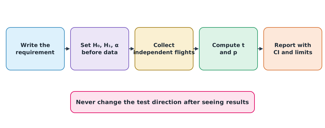
The requirement “mean endurance no less than 20 minutes with a 1.0 kg payload” needs evidence that the mean is greater than 20, so we set and , a one-sided test.
import pandas as pd

flights = pd.read_csv("endurance.csv")
a_1kg = flights.query("battery == 'A' and payload_kg == 1.0")["endurance_min"]
print("flights:", a_1kg.tolist())
res = stats.ttest_1samp(a_1kg, popmean=20, alternative="greater")
print(f"mean {a_1kg.mean():.3f}  t {res.statistic:.3f}  p {res.pvalue:.4f}  df {res.df}")
se = a_1kg.std() / math.sqrt(len(a_1kg))
print(f"one-sided 95% lower bound {a_1kg.mean() - stats.t.ppf(0.95, len(a_1kg) - 1) * se:.2f} min")
ci = stats.ttest_1samp(a_1kg, popmean=20).confidence_interval(0.95)
print(f"two-sided 95% CI [{ci.low:.2f}, {ci.high:.2f}] min")
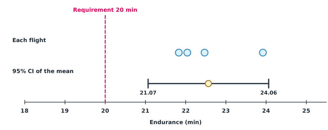
flights: [23.92, 22.04, 22.47, 21.83]
mean 22.565 t 5.447 p 0.0061 df 3
one-sided 95% lower bound 21.46 min
two-sided 95% CI [21.07, 24.06] minThe p-value is the probability of a result at least this extreme if were true. Here p = 0.006, below 0.05, so we reject : the data supports a mean above 20 minutes, and the one-sided 95% lower bound is about 21.46 minutes.
A passing mean does not mean every flight passes
A confidence interval describes uncertainty in the mean. The question “will 99% of flights exceed 20 minutes?” needs a tolerance interval, a different method in the NIST handbook that needs much more data. Conclusions from four flights also hold only for the battery, payload and weather tested.
Comparing two groups with Welch’s t-test
Next question: “does brand B fly longer than brand A with a 0.5 kg payload?” Use Welch’s t-test, which does not assume the two groups have equal spread. In SciPy you must pass equal_var=False, because the default assumes equal variances.
half = flights.query("payload_kg == 0.5")
a = half.query("battery == 'A'")["endurance_min"]
b = half.query("battery == 'B'")["endurance_min"]
res = stats.ttest_ind(b, a, equal_var=False)
ci = res.confidence_interval(0.95)
print(f"mean B - A = {b.mean() - a.mean():.2f} min   t {res.statistic:.3f}   p {res.pvalue:.3f}   df {res.df:.2f}")
print(f"95% CI of the difference [{ci.low:.2f}, {ci.high:.2f}] min")
mean B - A = 0.70 min t 1.015 p 0.353 df 5.36
95% CI of the difference [-1.04, 2.44] minWith p = 0.35, above 0.05, we do not reject , but we must not conclude that “the brands are equal”. The confidence interval for the difference, −1.04 to +2.44 minutes, shows that four flights per group are consistent both with B being about a minute worse and with it being almost two and a half minutes better. The honest answer is “the data cannot tell yet”.
Two kinds of error and how to use p-values
| true | false | |
|---|---|---|
| Reject | Type I error (chance ) | Correct (power) |
| Do not reject | Correct | Type II error |
import numpy as np

rng = np.random.default_rng(116)
null_true = rng.normal(20, 0.9, size=(10_000, 4))
p = stats.ttest_1samp(null_true, 20, axis=1, alternative="greater").pvalue
print(f"H0 true: rejected in {np.mean(p < 0.05):.1%} of 10 000 experiments")
for n in (4, 8, 16):
    real = rng.normal(21, 0.9, size=(10_000, n))
    p = stats.ttest_1samp(real, 20, axis=1, alternative="greater").pvalue
    print(f"true mean 21 min, n = {n:>2}: power {np.mean(p < 0.05):.1%}")
H0 true: rejected in 5.0% of 10 000 experiments
true mean 21 min, n = 4: power 52.1%
true mean 21 min, n = 8: power 87.7%
true mean 21 min, n = 16: power 99.5%When is true, a test at wrongly rejects about 5% of the time, as designed. When the true mean is 21 minutes, four flights detect it in only about half the experiments (52%). More flights raise the power, so plan the number of flights before testing.
The American Statistical Association (ASA) issued a statement on p-values in 2016. Its key principles include: a p-value does not measure the probability that a hypothesis is true; conclusions should not rest only on whether a p-value passes 0.05; reporting must be full and transparent; and a p-value does not measure the size of an effect. Always report the confidence interval of the difference alongside it.
Module lab
Lab: interpreting endurance tests
- Following lab guide L14 of the drone knowledge hub, write the requirement, hypotheses, direction and on the worksheet before opening
endurance.csv. - Test the “no less than 20 minutes” requirement for every brand and payload pair. Report the mean, SD, n, p-value and one-sided lower bound.
- Compare brands A and B at all three payloads with Welch’s t-test, and write conclusions that do not go beyond the data.
- Use simulation to find the smallest number of flights that gives 80% power when the true mean is 21 minutes and SD 0.9 minutes.
Common mistakes
Watch out
- Choosing one-sided or two-sided after seeing results so the p-value passes
- Using 1.96 with small samples: use the t value at degrees of freedom
- Concluding “equal” because was not rejected: finding no difference is not evidence of no difference
- Thinking the p-value is the chance that is true: it is computed assuming is already true
- Using the CI of the mean to certify every flight: that needs a tolerance interval
Summary
- SE , and the CI of the mean uses the value at degrees of freedom; small samples give wide intervals
- Set , , the direction and from the requirement before seeing data
- Compare two groups with Welch’s t-test, and report the CI of the difference alongside the p-value
- is the chance of a type I error, power grows with more data, and a p-value says nothing about the size or importance of an effect
Check your understanding
- A sample of 9 flights has minutes. What is the SE?
- For the requirement “noise no more than 70 dBA”, how should be set?
- What do you conclude from p = 0.03 at ?
- A test gives p = 0.40 and the author writes “proven to be no different”. What is wrong?
- Why must SciPy’s
ttest_indbe givenequal_var=Falsefor a Welch’s t-test?
Answers
- minutes
- dBA, because we need evidence that noise is below the limit ()
- Reject ; the data supports at the 0.05 level, and the confidence interval should be reported too
- Not rejecting is not evidence of equality; the data may simply be too small. Report the confidence interval of the difference
- Because the default of
ttest_indisequal_var=True, which assumes the two groups have equal variance
Key formulas
| Standard error of the mean | |
| Two-sided confidence interval for the mean | |
| One-sample t statistic | |
| Welch t statistic |
Key references
- Montgomery, D. C., & Runger, G. C. (2018). Applied statistics and probability for engineers (7th ed.). Wiley. link
- NIST/SEMATECH. Confidence limits for the mean (section 1.3.5.2). e-Handbook of statistical methods. link
- NIST/SEMATECH. Two-sample t-test for equal means (section 1.3.5.3). e-Handbook of statistical methods. link
- NIST/SEMATECH. Tolerance intervals for a normal distribution (section 7.2.6.3). e-Handbook of statistical methods. link
- The SciPy community. Statistical functions (scipy.stats), SciPy 1.18 documentation. link
- Wasserstein, R. L., & Lazar, N. A. (2016). The ASA statement on p-values: Context, process, and purpose. The American Statistician, 70(2), 129–133. link
- Diez, D. M., Çetinkaya-Rundel, M., & Barr, C. D. (2019). OpenIntro statistics (4th ed.). OpenIntro. link
Further reading
Study the assigned knowledge units in advance, review media and take the module quiz
In class / field
Lab or field practice from worksheets with a safety checklist
Learning evidence: Checked worksheets and quiz results