Probability and distributions
UAT 106 Statistics and Data Analytics for Technology
Lesson
By the end of this module you will be able to
- Apply the addition and multiplication rules, conditional probability and Bayes' theorem
- Calculate probabilities from the binomial and normal distributions with SciPy
- Convert values to z-scores and use the 68–95–99.7 rule to assess data
- Run seeded Monte Carlo simulations and explain the central limit theorem
Why this matters
“95% mission success” sounds good, but if a unit flies 20 missions a week, some week is very likely to include a failure. Probability turns risk figures into terms that match real use, and the distribution of data answers questions such as “what is the chance this battery flies less than 20 minutes?”, which is the basis of testing in module 3.
Basic rules of probability
A probability is a number from 0 to 1 that says how likely an event is.
- Complement:
- Independent events: one outcome does not change the chance of the other, so probabilities multiply:
- Conditional probability is the chance of given that has happened
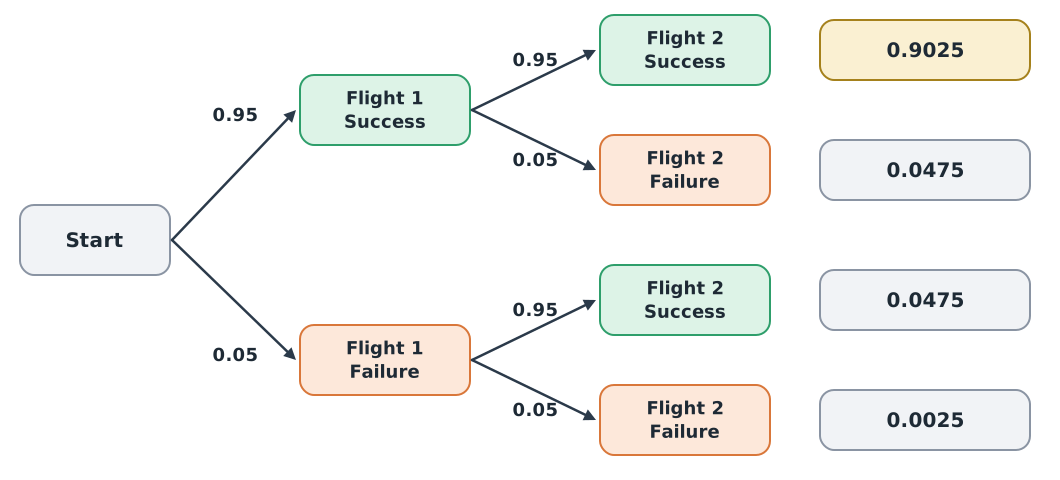
The chance that both flights succeed is , and the four leaves always add up to 1. Multiplying like this only works when flights really are independent. If failures share a cause, such as a windy day or a bug in one software version, flights are not independent.
The binomial distribution
When a trial is repeated times, each ending in success or failure with a fixed chance, and each trial is independent, the number of failures follows a binomial distribution.
from scipy import stats

n, p_fail = 20, 0.05
print(f"P(at least one failure in {n} flights) = {1 - 0.95 ** n:.4f}")
failures = stats.binom(n, p_fail)
for k in range(4):
    print(f"P(X = {k}) = {failures.pmf(k):.4f}")
print(f"P(X >= 2) = {failures.sf(1):.4f}   expected failures = {failures.mean():.1f}")
P(at least one failure in 20 flights) = 0.6415
P(X = 0) = 0.3585
P(X = 1) = 0.3774
P(X = 2) = 0.1887
P(X = 3) = 0.0596
P(X >= 2) = 0.2642 expected failures = 1.0Even though each flight succeeds 95% of the time, 20 flights have a 64% chance of at least one failure, and one failure is expected on average. That helps plan spares and emergency procedures.
Example 1 A motor alarm and Bayes’ theorem
A vibration monitor raises an alarm when it suspects a failing motor. Suppose 2% of motors are really faulty, the alarm catches 90% of faulty motors (its sensitivity), but it also falsely alarms on 5% of healthy motors. If the alarm sounds, what is the chance the motor is really faulty?
p_fault = 0.02
p_alarm_if_fault = 0.90
p_alarm_if_ok = 0.05
p_alarm = p_alarm_if_fault * p_fault + p_alarm_if_ok * (1 - p_fault)
p_fault_if_alarm = p_alarm_if_fault * p_fault / p_alarm
print(f"P(alarm) = {p_alarm:.4f}   P(fault | alarm) = {p_fault_if_alarm:.3f}")
P(alarm) = 0.0670 P(fault | alarm) = 0.269Although the monitor is 90% sensitive, an alarm means a real fault only about 27% of the time, because healthy motors are far more numerous, so false alarms outnumber true ones. An alarm should lead to confirmation checks, not an immediate motor swap.
The normal distribution
Data produced by many small effects added together, such as endurance influenced by wind, temperature and battery condition, often looks like the normal distribution, a symmetric bell curve defined by its mean and standard deviation .
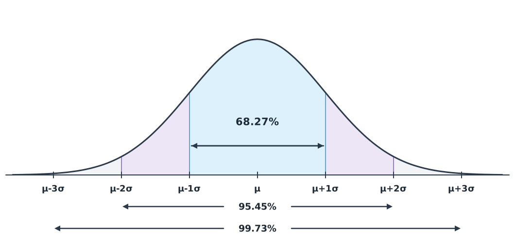
A z-score says how many a value lies from the mean. For a normal distribution about 68.27% of data lies within , 95.45% within and 99.73% within : the 68–95–99.7 rule.
for k in (1, 2, 3):
    print(f"within ±{k} sigma: {stats.norm.cdf(k) - stats.norm.cdf(-k):.4%}")

mu, sigma = 23.0, 1.5
print(f"z of 20 min = {(20 - mu) / sigma:.1f}   P(endurance < 20 min) = {stats.norm.cdf(20, mu, sigma):.4f}")
print(f"99% of flights last at least {stats.norm.ppf(0.01, mu, sigma):.2f} min")
within ±1 sigma: 68.2689%
within ±2 sigma: 95.4500%
within ±3 sigma: 99.7300%
z of 20 min = -2.0 P(endurance < 20 min) = 0.0228
99% of flights last at least 19.51 minIf a battery model’s endurance is normal with mean 23 minutes and SD 1.5 minutes, the 20-minute requirement lies 2 SD below the mean, so a flight falls short about 2.3% of the time. norm.cdf gives the area to the left of a value; norm.ppf does the reverse, finding the value for a given area.
Real data is not always normal
The processing times in module 1 are clearly right-skewed. Applying normal-distribution formulas to data like that underestimates how often slow frames occur. Always look at a histogram before choosing a model.
Monte Carlo simulation and the central limit theorem
When formulas get hard, we simulate the situation with many random numbers and count the outcomes: Monte Carlo simulation. Always set a seed for the random number generator so results repeat.
import numpy as np

rng = np.random.default_rng(116)
flights = rng.normal(mu, sigma, size=100_000)
print(f"simulated P(< 20 min) = {np.mean(flights < 20):.4f}   exact = {stats.norm.cdf(20, mu, sigma):.4f}")

pairs = rng.normal(mu, sigma, size=(100_000, 2))
both_ok = np.mean((pairs >= 20).all(axis=1))
print(f"two batteries both reach 20 min: simulated {both_ok:.4f}   exact {(1 - stats.norm.cdf(20, mu, sigma)) ** 2:.4f}")
simulated P(< 20 min) = 0.0234 exact = 0.0228
two batteries both reach 20 min: simulated 0.9550 exact 0.9550The simulation is close to the formula and gets closer with more runs. The method works for far more complex problems, such as multi-stage missions where each stage has its own distribution.
The central limit theorem says that when we average enough independent samples, the mean is close to normally distributed even if the original data is not, and its standard deviation shrinks to .
import pandas as pd

lat = pd.read_csv("latency.csv")["latency_ms"].to_numpy()
means = rng.choice(lat, size=(20_000, 25)).mean(axis=1)
print(f"data: sd {lat.std(ddof=1):.2f} ms, skew {stats.skew(lat):.2f}")
print(f"means of 25 frames: sd {means.std(ddof=1):.2f} ms (sigma/sqrt(25) = {lat.std(ddof=1) / 5:.2f}), skew {stats.skew(means):.2f}")
data: sd 11.41 ms, skew 0.78
means of 25 frames: sd 2.30 ms (sigma/sqrt(25) = 2.28), skew 0.18The processing times are right-skewed (clearly positive skew), but means of 25 frames are much less skewed and about five times less spread, as predicts. This is why module 3 can build confidence intervals from the distribution of the mean.
Module lab
Lab: assessing mission risk
- A unit flies 50 missions a month, each with a 1% chance of an emergency landing. Find the chance of a month with none, and of more than 2, using both the formula and simulation.
- Change the motor-alarm example so that 10% of motors are faulty, and explain why changes so much.
- Plot a histogram of
hover_error.csvagainst a normal curve with the same mean and SD, then test it withscipy.stats.shapiro. Remove the outliers and test again. - Simulate a mission of three consecutive legs, each with its own normally distributed duration, and find the chance that the total exceeds 60 minutes.
Common mistakes
Watch out
- Multiplying probabilities of dependent events, such as flights on the same windy day
- Confusing with : an alarm’s sensitivity is not the chance that an alarm means a real fault
- Using the normal distribution on skewed data without looking at its shape first
- Simulating without a seed, so results change every run and nobody can check them
- Thinking the central limit theorem makes the original data normal: it is about means, not individual values
Summary
- Probabilities of independent events multiply; conditional probabilities need Bayes’ theorem
- The binomial distribution counts successes or failures in repeated independent trials
- The normal distribution is set by and ; z-scores and the 68–95–99.7 rule apply when data is close to normal
- Monte Carlo simulation needs a seed, and sample means approach normality under the central limit theorem
Check your understanding
- Three drones fly at once, each with an independent 2% chance of a fault. What is the chance that none has a fault?
- Ten flights, each failing 10% of the time. How many failures are expected on average?
- Mean endurance is 25 minutes with SD 2 minutes. What is the z-score of 21 minutes?
- For normal data, about what percentage lies outside ?
- Data has ms. What is the approximate standard deviation of the mean of a sample of 36?
Answers
- flight
- ms
Key formulas
| Multiplication rule for independent events | |
| Bayes' theorem | |
| Binomial distribution | |
| z-score | |
| Standard deviation of the mean |
Key references
- Montgomery, D. C., & Runger, G. C. (2018). Applied statistics and probability for engineers (7th ed.). Wiley. link
- Diez, D. M., Çetinkaya-Rundel, M., & Barr, C. D. (2019). OpenIntro statistics (4th ed.). OpenIntro. link
- NIST/SEMATECH. Normal distribution (section 1.3.6.6.1). e-Handbook of statistical methods. link
- The SciPy community. Statistical functions (scipy.stats), SciPy 1.18 documentation. link
- NIST/SEMATECH. e-Handbook of statistical methods. National Institute of Standards and Technology. link
- Python Software Foundation. statistics — Mathematical statistics functions. The Python standard library (3.14). link
Further reading
Study the assigned knowledge units in advance, review media and take the module quiz
In class / field
Lab or field practice from worksheets with a safety checklist
Learning evidence: Checked worksheets and quiz results