Control experiments in SITL
UAT 206 Fundamentals of Control and Autopilot Systems
Lesson
By the end of this module you will be able to
- Set up control experiments in PX4 or ArduPilot SITL and collect logs
- Compute rise time, overshoot and settling time from step-response data
- Compare two tuning sets systematically
- Measure path-tracking error with simulated wind
Why this matters
Tuning on a real drone risks a crash, and the same conditions are hard to repeat. SITL (software in the loop) runs the real autopilot software on a computer connected to a simulator, so gains can be changed safely and results compared fairly. The drone knowledge base’s SITL unit stresses getting a basic setup working first, then adding other parts one at a time, and recording versions and logs every time.
Experiment architecture
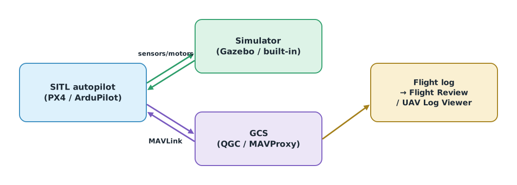
The SITL autopilot receives sensor values from the simulator and sends motor commands back. The GCS connects over MAVLink to command and monitor, and logs are analysed with PX4’s Flight Review or ArduPilot’s UAV Log Viewer. The PX4 guide uses make px4_sitl gz_x500 to start a quadcopter in Gazebo, and ArduPilot has a built-in SITL that does not need Gazebo.
Measuring step responses from logs
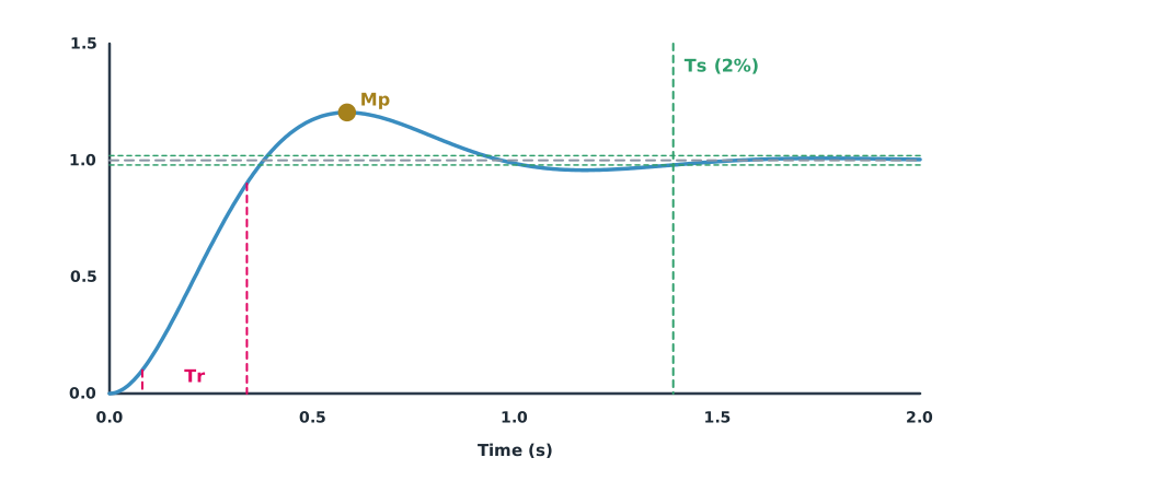
The PX4 tuning guide tests with step inputs while hovering, and the Flight Review page says the estimate should closely follow the setpoint; if not, the gains need tuning. Looking at plots helps, but computing metrics makes comparing two tuning sets clear.
Example 1 Comparing two tuning sets from a rate log
A simulated log of roll-rate response to a step command, recorded at 250 Hz. Set A has high P; set B has lower P and more D.
import math

def response(zeta, w0, rate_hz=250, t_end=2.0):
    t = [k / rate_hz for k in range(int(t_end * rate_hz))]
    wd = w0 * math.sqrt(1 - zeta ** 2)
    y = [1 - math.exp(-zeta * w0 * s) * (math.cos(wd * s) + zeta / math.sqrt(1 - zeta ** 2) * math.sin(wd * s)) for s in t]
    return t, y

def metrics(t, y, target=1.0):
    t10 = next(a for a, b in zip(t, y) if b >= 0.1 * target)
    t90 = next(a for a, b in zip(t, y) if b >= 0.9 * target)
    over = max(y) / target - 1
    ts = next(t[i] for i in range(len(y)) if all(abs(v - target) <= 0.02 * target for v in y[i:]))
    return t90 - t10, over, ts

for name, zeta, w0 in (("set A (high P)", 0.45, 6.0), ("set B (lower P, more D)", 0.7, 5.0)):
    tr, mp, ts = metrics(*response(zeta, w0))
    print(f"{name:<24} rise {tr * 1000:4.0f} ms, overshoot {mp:5.1%}, settling {ts:.2f} s")
set A (high P) rise 256 ms, overshoot 20.5%, settling 1.39 s
set B (lower P, more D) rise 424 ms, overshoot 4.6%, settling 1.20 sSet A rises faster but overshoots by about a fifth and settles slowly. Set B rises more slowly but barely overshoots and settles sooner, closer to what the PX4 guide asks for. With a real log, trim the part before the command and use the actual final value instead of 1.0.
Tracking error with wind
Lab L02 in the drone knowledge base flies the same mission without and with wind, changing one variable only, and compares errors on the same axis and units. The usual figures to report are RMS and maximum.
Example 2 Path-tracking error
Cross-track error along a straight 60 s path recorded at 10 Hz (hypothetical data).
import math

t = [k / 10 for k in range(600)]
calm = [0.15 * math.sin(0.8 * s) for s in t]                               # m no wind
windy = [0.8 * (1 - math.exp(-s / 5)) + 0.3 * math.sin(0.5 * s) for s in t]  # m crosswind

def summary(err):
    rms = math.sqrt(sum(e * e for e in err) / len(err))
    return rms, max(abs(e) for e in err), sum(err) / len(err)

for name, err in (("calm", calm), ("crosswind", windy)):
    rms, peak, bias = summary(err)
    print(f"{name:<10} RMS {rms:.2f} m, max {peak:.2f} m, mean offset {bias:+.2f} m")
calm RMS 0.11 m, max 0.15 m, mean offset +0.01 m
crosswind RMS 0.78 m, max 1.10 m, mean offset +0.74 mA crosswind gives the error a mean offset to one side, showing that the velocity loop is not fully rejecting a constant disturbance. If raising the velocity loop’s I reduces the mean, that is the right fix. After tuning by hand, compare with PX4 Autotune or ArduPilot AutoTune, which the guides recommend running around hover.
Module lab
Lab: tuning and testing in SITL
- Start SITL following the PX4 (Gazebo) or ArduPilot guide, recording firmware version, simulator version and parameter file.
- Command a roll step while hovering, open the log in Flight Review or UAV Log Viewer and export the rate data.
- Apply the
metricsfunction from Example 1 to real data for two tuning sets. - Fly a straight-line mission with and without wind following lab L02, and compute the errors with Example 2.
- Write a short report comparing the tuning sets, with plots, parameter files and the limits of simulation results.
Common mistakes
Watch out
- Changing several values in one experiment.
- Not recording software versions and parameter files.
- Assuming good SITL gains work on the real drone straight away.
- Judging plots by eye only without computing metrics.
- Comparing results over different time spans or units.
Summary
- SITL runs real autopilot software with a simulator, so experiments are safe and repeatable.
- Measure , and from logs to compare tuning sets numerically.
- Report tracking error as RMS, maximum and mean.
- SITL results must be confirmed with careful real flights before use.
Check your understanding
- How does SITL differ from flying in an ordinary simulator game?
- The response reaches 10% at 0.05 s and 90% at 0.17 s. What is the rise time?
- The response peaks at 1.25 with a final value of 1.0. What is the overshoot?
- What is the RMS of errors 0.3, −0.4 and 0 m?
- What does a non-zero mean error in a crosswind tell you?
Answers
- SITL runs the same autopilot software used on the drone.
- s
- 25%.
- m
- The controller is not fully rejecting a constant disturbance; the velocity loop’s I may need raising.
Key formulas
| RMS tracking error |
Key references
- PX4 Autopilot. Gazebo simulation. PX4 user guide (main). link
- ArduPilot Dev Team. SITL simulator (software in the loop). link
- PX4 Autopilot. Log analysis using Flight Review. PX4 guide (main). link
- ArduPilot Dev Team. UAV Log Viewer. ArduPilot Copter documentation. link
- PX4 Autopilot. Multicopter PID tuning guide. PX4 guide (main). link
- PX4 Autopilot. Multicopter auto-tuning. PX4 guide (main). link
- ArduPilot Dev Team. AutoTune. ArduPilot Copter documentation. link
- Åström, K. J., & Murray, R. M. (2021). Feedback systems: An introduction for scientists and engineers (2nd ed.). Princeton University Press. link
Further reading
Study the assigned knowledge units in advance, review media and take the module quiz
Holding a track in simulated wind
Developing simulations and connecting SITL
In class / field
Lab or field practice from worksheets with a safety checklist
Learning evidence: Checked worksheets and quiz results