Module 4/5 · Weeks 10–12 · 27 h

Deep learning and object detection

UAT 306 Artificial Intelligence for UAS

About 90 minDraft, awaiting reviewLast updated 28 September 2026

By the end of this module you will be able to

Compute the output size and parameter count of convolution layers
Explain how an object detector predicts both class and location
Write non-maximum suppression to remove duplicate boxes
Compute a detector's precision, recall and average precision

Prerequisites: UAT 306 Modules 1–3

Why this matters

The drone knowledge base’s unit on deep learning and CNNs covers neural networks, CNNs, transfer learning and object detection. Its unit on training and evaluating object detection explains that a detector must predict both the type and location of objects, that IoU is used to match predictions to answers, and that mAP combines ranking with several conditions. This module computes these key pieces by hand, step by step, so that the output of tools such as Ultralytics YOLO can be read with understanding.

Convolution layers

A convolution layer slides a $k \times k$ filter over the image, and the accumulated products form a feature map. The output size depends on the input size $i$ , kernel size $k$ , padding $p$ and stride $s$ , following the formula in A guide to convolution arithmetic (Dumoulin and Visin, 2016). Each filter has $k \times k \times C_{in}$ weights plus one bias, and a layer has $C_{out}$ filters.

Example 1 Size and parameters of early layers

def conv_out(i, k, s, p):
    return (i + 2 * p - k) // s + 1

def conv_params(k, c_in, c_out):
    return k * k * c_in * c_out + c_out

print("640 px, k=3, s=1, p=1 ->", conv_out(640, 3, 1, 1))
print("640 px, k=3, s=2, p=1 ->", conv_out(640, 3, 2, 1))
print("layer 3x3, RGB -> 32 channels:", conv_params(3, 3, 32), "parameters")
print("layer 3x3, 32 -> 64 channels:", conv_params(3, 32, 64), "parameters")
full = 640 * 640 * 3 * 32
print(f"a fully connected layer from a 640x640 RGB image to 32 outputs would need {full:,} weights")

640 px, k=3, s=1, p=1 -> 640
640 px, k=3, s=2, p=1 -> 320
layer 3x3, RGB -> 32 channels: 896 parameters
layer 3x3, 32 -> 64 channels: 18496 parameters
a fully connected layer from a 640x640 RGB image to 32 outputs would need 39,321,600 weights

A convolution layer has very few parameters compared with a fully connected layer, because it reuses the same filters across the image. A stride of 2 halves the image size, so detection networks shrink their feature maps step by step to see wider context.

Removing duplicates with NMS

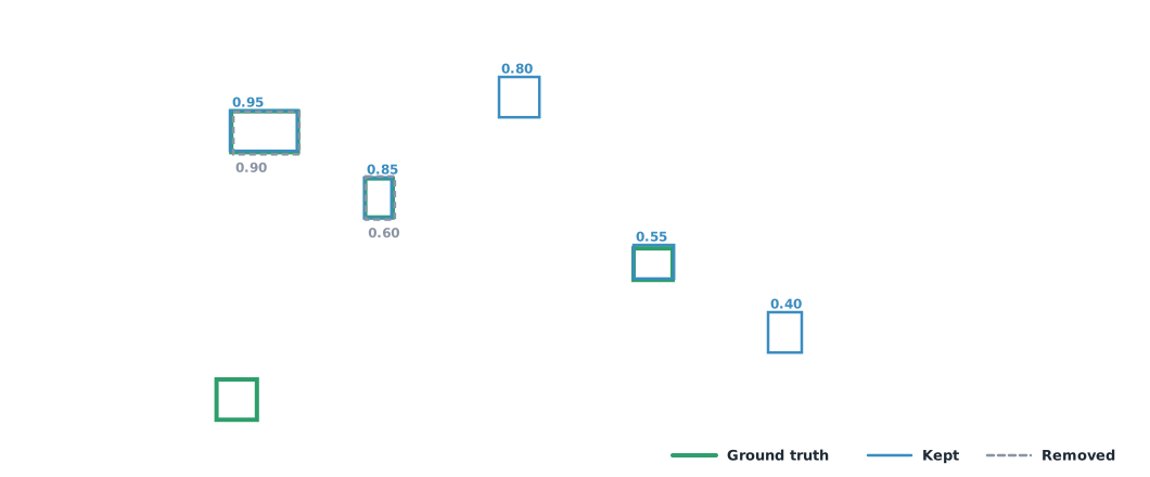
Detectors often predict several boxes around the same object. Greedy non-maximum suppression (NMS) keeps the highest-scoring box, removes other boxes that overlap it by more than a set IoU, and repeats until none are left. This approach was used in R-CNN (Girshick et al., 2014) and is available in libraries such as torchvision.ops.nms.

Precision, recall and AP

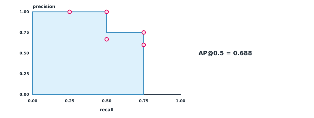
When matching predictions to ground truth, a prediction whose IoU with a ground-truth box exceeds 0.5 counts as correct (a true positive) under the PASCAL VOC criterion (Everingham et al., 2010). Matching proceeds in order of decreasing score, each ground-truth box can be matched only once, and duplicate predictions count as false. Cumulative precision and recall are then computed. Average precision (AP) summarises the precision–recall curve as one number. The VOC paper averages precision at 11 recall levels, while COCO uses 101 levels and averages over IoU 0.50 to 0.95 (Lin et al., 2014), which is stricter. This example computes the area under the curve at every point after making precision non-increasing as recall falls.

Example 2 NMS and then AP at IoU 0.5

One image has 4 cracks, and the detector predicts 7 boxes (simulated data).

import numpy as np

def iou(p, q):
    ix = max(0, min(p[2], q[2]) - max(p[0], q[0]))
    iy = max(0, min(p[3], q[3]) - max(p[1], q[1]))
    inter = ix * iy
    return inter / ((p[2] - p[0]) * (p[3] - p[1]) + (q[2] - q[0]) * (q[3] - q[1]) - inter)

dets = [(0.95, (100, 100, 200, 160)), (0.90, (105, 102, 203, 165)), (0.85, (300, 200, 340, 260)),
        (0.80, (500, 50, 560, 110)), (0.60, (302, 198, 345, 262)), (0.55, (700, 300, 760, 350)),
        (0.40, (900, 400, 950, 460))]
gts = [(102, 101, 201, 162), (301, 201, 342, 259), (700, 305, 758, 352), (80, 500, 140, 560)]

kept = []
for score, box in sorted(dets, reverse=True):          # greedy NMS
    if all(iou(box, k) < 0.5 for _, k in kept):
        kept.append((score, box))
print("after NMS:", [s for s, _ in kept])

used, tp = set(), []
for score, box in kept:
    g = max(range(len(gts)), key=lambda j: iou(box, gts[j]))
    hit = iou(box, gts[g]) > 0.5 and g not in used
    used.add(g) if hit else None
    tp.append(hit)
ctp = np.cumsum(tp)
prec = ctp / np.arange(1, len(tp) + 1)
rec = ctp / len(gts)
for s, p, r in zip([s for s, _ in kept], prec, rec):
    print(f"score {s:.2f}: precision {p:.2f}, recall {r:.2f}")
p_interp = np.maximum.accumulate(prec[::-1])[::-1]
ap = np.sum(np.diff(np.r_[0, rec]) * p_interp)
print(f"AP@0.5 = {ap:.3f}")

after NMS: [0.95, 0.85, 0.8, 0.55, 0.4]
score 0.95: precision 1.00, recall 0.25
score 0.85: precision 1.00, recall 0.50
score 0.80: precision 0.67, recall 0.50
score 0.55: precision 0.75, recall 0.75
score 0.40: precision 0.60, recall 0.75
AP@0.5 = 0.688

NMS removes the two duplicate boxes that overlap higher-scoring boxes. Then 3 of 5 predictions are correct and 3 of 4 cracks are found. AP is below 1 because a high-scoring false prediction sits among the correct ones and one crack is never detected. Real tools compute AP over every image in the test set together, and tools may approximate the area slightly differently, so always state the criterion when reporting.

Precision against recall from 0 to 1: a blue step curve from precision 1.0 at recall 0.25 and 0.5, falling when false predictions appear; the shaded light blue area under the curve is the AP of about 0.69 — Figure 1 Precision–recall curve and AP area

A simulated image with seven predicted boxes: blue boxes are kept after NMS, grey dashed boxes are removed duplicates, and green boxes are the four real cracks — Figure 2 Boxes kept and removed by NMS

Module lab

Lab: training and evaluating a detector

Compute the feature-map sizes of the first three layers of the model you will use, with Example 1
Train a detector (such as a small YOLO) on the dataset from Module 3 with transfer learning
Export predictions on the validation set, compute AP@0.5 with Example 2 and compare with the tool’s value
Change the NMS IoU and the confidence threshold and observe precision and recall
Look at the wrong predictions one by one and group the causes

Common mistakes

Watch out

Comparing AP under different criteria, such as AP@0.5 and AP@0.5:0.95
Forgetting NMS and counting duplicate boxes as detections
Looking only at mAP without examining the wrong images
Training from scratch with little data instead of using transfer learning
Using images that are too small, so small cracks disappear after resizing

Summary

Convolution output size is $⌊(i + 2 p - k) / s ⌋ + 1$ , and the parameter count does not depend on image size
NMS keeps the highest-scoring box and removes boxes that overlap it beyond the set IoU
A prediction is correct when its IoU with an unmatched ground truth exceeds 0.5 (VOC criterion); AP summarises the precision–recall curve
Always report AP with its IoU criterion and method

Check your understanding

Input 320, kernel 3, stride 2, padding 1. What is the output size?
How many parameters does a 3×3 layer from 64 to 128 channels have?
Two boxes have IoU 0.7. How many does NMS at 0.5 keep?
Two predictions both have IoU above 0.5 with the same ground truth. How are they counted?
Why is COCO AP usually lower than AP@0.5?

Answers

$⌊(320 + 2 - 3) /2 ⌋ + 1 = 160$
$3 \times 3 \times 64 \times 128 + 128 = 73, 856$
One (the higher-scoring box)
The first is correct and the second is false
It averages over IoU 0.50 to 0.95, and the higher thresholds demand much more precise boxes

Key formulas

Convolution output size	$o = ⌊ \frac{i + 2 p - k}{s} ⌋ + 1$
Parameters of a convolution layer	$N = k \times k \times C_{in} \times C_{out} + C_{out}$
Average precision	$A P = \sum_{n} (r_{n} - r_{n - 1}) p_{interp} (r_{n})$

Key references

Prince, S. J. D. (2023). Understanding deep learning. MIT Press. link
Géron, A. (2022). Hands-on machine learning with Scikit-Learn, Keras, and TensorFlow (3rd ed.). O'Reilly.
Dumoulin, V., & Visin, F. (2016). A guide to convolution arithmetic for deep learning (arXiv:1603.07285). link
Girshick, R., Donahue, J., Darrell, T., & Malik, J. (2014). Rich feature hierarchies for accurate object detection and semantic segmentation. In 2014 IEEE Conference on Computer Vision and Pattern Recognition (pp. 580–587). link
PyTorch Contributors. torchvision.ops.nms. Torchvision documentation. link
Everingham, M., Van Gool, L., Williams, C. K. I., Winn, J., & Zisserman, A. (2010). The PASCAL visual object classes (VOC) challenge. International Journal of Computer Vision, 88(2), 303–338. link
Lin, T.-Y., Maire, M., Belongie, S., Hays, J., Perona, P., Ramanan, D., Dollár, P., & Zitnick, C. L. (2014). Microsoft COCO: Common objects in context. In Computer Vision – ECCV 2014 (pp. 740–755). Springer. link

In class / field

Lab or field practice from worksheets with a safety checklist

Learning evidence: Checked worksheets and quiz results

Module quiz

This is a formative self-check, not a graded exam

Knowledge domain: Artificial intelligence and computer vision

Deep learning and object detection

By the end of this module you will be able to

Why this matters

Convolution layers

Removing duplicates with NMS

Precision, recall and AP

Module lab

Common mistakes

Summary

Check your understanding

Key formulas

Key references

Further reading

Deep learning and CNNs

Training and evaluating object detection

Ultralytics YOLO

In class / field

Module quiz

Deep learning and object detection

Lesson

By the end of this module you will be able to

Why this matters

Convolution layers

Removing duplicates with NMS

Precision, recall and AP

Module lab

Common mistakes

Summary

Check your understanding

Key formulas

Key references

Further reading

Deep learning and CNNs

Training and evaluating object detection

Ultralytics YOLO

In class / field

Module quiz