Digital images and cameras

Why this matters

UAT 315 used OpenCV to find objects by colour and track them, and UAT 205 covered the pinhole camera model and calibration. This course goes deeper into the algorithms behind frequently used functions, so that you can choose and adjust them when real drone images differ from sample images. The drone knowledge base’s unit on computer vision and Edge AI lays these foundations, and its OpenCV unit demonstrates colour, thresholding and edge detection. The textbooks by Szeliski and Corke explain these algorithms in detail. The examples use synthetic data so that answers can be checked.

An image is an array of numbers

An 8-bit greyscale image is a two-dimensional array of values 0–255; a colour image has three channels; a radiometric thermal image stores values that convert to temperature. Quantising to 8 bits loses detail in very dark or very bright areas, and lossy compression adds block noise. Every processing step must therefore know what kind of source data it has.

Edge detection with Sobel

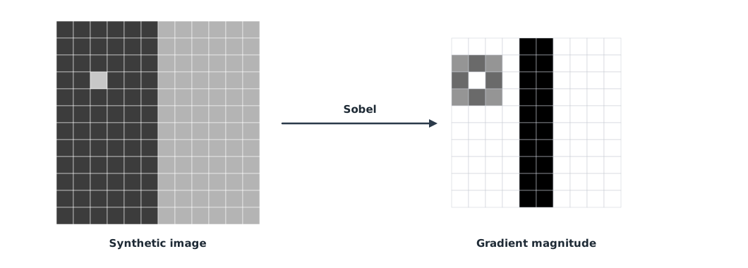
An edge is where brightness changes quickly. The Sobel filter is a 3×3 kernel that approximates the horizontal derivative $G_x$ and vertical derivative $G_y$, which combine into the gradient magnitude. In drone work it finds crack edges, road lines or roof edges. OpenCV provides cv2.Sobel; this example writes the convolution by hand to show the computation.

import numpy as np

img = np.full((12, 12), 60.0)
img[:, 6:] = 180.0
img[3, 2] = 200.0                               # noise pixel
kx = np.array([[-1, 0, 1], [-2, 0, 2], [-1, 0, 1]])
ky = kx.T

def conv(a, k):
    out = np.zeros((a.shape[0] - 2, a.shape[1] - 2))
    for i in range(out.shape[0]):
        for j in range(out.shape[1]):
            out[i, j] = (a[i:i + 3, j:j + 3] * k).sum()
    return out

mag = np.hypot(conv(img, kx), conv(img, ky))
print(f"largest gradient {mag.max():.0f} at output columns {sorted(set(np.argwhere(mag == mag.max())[:, 1]))}")
strong = mag > 200
print(f"pixels above 200: {strong.sum()} (edge columns {sorted(set(np.argwhere(strong)[:, 1]))})")

largest gradient 480 at output columns [np.int64(4), np.int64(5)]
pixels above 200: 24 (edge columns [np.int64(0), np.int64(1), np.int64(2), np.int64(4), np.int64(5)])

Choosing a threshold with Otsu’s method

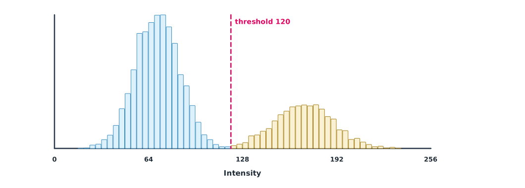
Separating objects from background with a single threshold requires a good choice. Otsu’s method (1979) tries every threshold and chooses the one that maximises the between-class variance ${\sigma }_B^2$, which is equivalent to minimising the weighted within-class variance as the OpenCV tutorial explains. OpenCV applies it through cv2.threshold with the THRESH_OTSU flag.

import numpy as np

rng = np.random.default_rng(3)
pix = np.r_[rng.normal(70, 15, 7000), rng.normal(170, 20, 3000)].clip(0, 255).astype(int)
p = np.bincount(pix, minlength=256) / pix.size
best_var, best_t = 0.0, 0
for t in range(1, 256):
    w0, w1 = p[:t].sum(), p[t:].sum()
    if w0 == 0 or w1 == 0:
        continue
    m0 = (np.arange(t) * p[:t]).sum() / w0
    m1 = (np.arange(t, 256) * p[t:]).sum() / w1
    var_b = w0 * w1 * (m0 - m1) ** 2
    if var_b > best_var:
        best_var, best_t = var_b, t
print(f"Otsu threshold {best_t}, bright fraction {(pix >= best_t).mean():.1%} (true roof fraction 30%)")

Otsu threshold 120, bright fraction 29.9% (true roof fraction 30%)

Module lab

Common mistakes

Summary

• A digital image is an array of numbers; know the source data type before processing
• Sobel approximates the brightness derivative; high gradient magnitude marks edges but is sensitive to noise
• Otsu chooses the threshold that maximises between-class variance and suits two-peaked histograms
• Uneven lighting needs local methods

Check your understanding

1. How many levels does an 8-bit image have?
2. With background 60 and edge value 180, what is the largest horizontal Sobel response at a vertical edge?
3. Why does one noise pixel create edges in several pixels?
4. What criterion does Otsu’s method use to choose the threshold?
5. If half the image has cloud shadow, which kind of threshold should be used?