Photogrammetry and outputs
UAT 361 Unmanned Aircraft Systems Technology for Surveying, Mapping and Inspection
Lesson
By the end of this module you will be able to
- Explain how depth comes from parallax when the camera moves, and compute depth from parallax
- Explain the Structure from Motion workflow and bundle adjustment, and what reprojection error means
- Choose orthomosaic, point cloud, mesh, DSM and DTM outputs to match the user's question
- Compute stockpile volume from a height grid and disclose areas with no data
Why this matters
Modern mapping software produces attractive results at the press of a button. But when the map splits into two blocks, a stockpile has holes, or the user asks for “ground height” under trees, someone who does not understand how images become maps cannot fix the problem, and may deliver files with the right names but the wrong meaning. This module explains as much of the mechanism as you need to make those decisions.
Depth comes from parallax
One photograph gives the direction from the camera to an object but not its distance. When the camera moves, the same point appears at a different position in the image. This is parallax. Hold a finger in front of your face and close each eye in turn: the nearby finger jumps more than distant objects. Photogrammetry uses the same principle.
For an image pair taken at the same height a distance apart (the base), the photogrammetry textbook by Wolf and colleagues gives , where is the parallax on the image plane.
Example 1. Roof height from parallax
Using the camera and flight plan from module 1: base 16 m, = 8.8 mm, pixel size 13.2/5472 mm.
BASE_M, FOCAL_MM = 16.0, 8.8
PIXEL_MM = 13.2 / 5472

def depth_m(parallax_px):
    return BASE_M * FOCAL_MM / (parallax_px * PIXEL_MM)

ground_px, roof_px = 729.6, 810.7
z_ground, z_roof = depth_m(ground_px), depth_m(roof_px)
print(f"ground {z_ground:.1f} m below camera, roof {z_roof:.1f} m, roof height {z_ground - z_roof:.1f} m")
print(f"1 px parallax error at 80 m changes depth by about {80 ** 2 / (BASE_M * FOCAL_MM) * PIXEL_MM:.2f} m")
ground 80.0 m below camera, roof 72.0 m, roof height 8.0 m
1 px parallax error at 80 m changes depth by about 0.11 mA parallax difference of about 81 pixels shows the roof is about 8 m high. A parallax error of a single pixel changes depth by almost 11 cm, so heights are usually less accurate than horizontal positions, and a longer base relative to height makes depth more precise.
Structure from Motion
A drone survey uses hundreds of images, not one pair. Structure from Motion (SfM) estimates the position and orientation of every camera together with the shape of the scene. The method grew out of computer vision work such as Snavely and colleagues (2006) and has been widely adopted in the geosciences, as reviewed by Westoby and colleagues (2012).
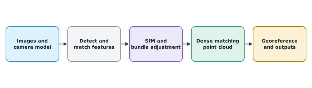
- Images and camera model: read the image size, focal length and lens distortion
- Detect and match features: for example, corners of marks on the ground. Points tracked across several images are tie points; matches that conflict with the geometry are rejected
- SfM and bundle adjustment: OpenSfM starts from an initial image pair, adds images one at a time, computes 3D points and periodically refines everything together with bundle adjustment, so that points projected back into the images land as close as possible to where they are seen
- Dense matching: estimate depth for many pixels, giving a dense point cloud
- Georeference and outputs: use camera positions or GCPs, then create the orthomosaic, DSM or mesh
Reprojection error measures how many pixels a point projected back into an image lies from where it is seen. It is internal consistency, not error on the ground. A model with low reprojection error can still be shifted as a whole if the georeferencing is wrong.
A map split into two blocks
If the middle of the site is a pond reflecting the sky, or a roof with a repeating pattern, the software may fail to match across the two sides. Adding more points in dense matching does not help, because it cannot create linking images that do not exist. Check the images at the seam and, if needed, fly more images along edges with stable surfaces.
Five kinds of output
| Output | Data held | Answers | Watch for |
|---|---|---|---|
| Orthomosaic | Mosaic corrected for camera angle and terrain, with coordinates | What is where, and how large? | Building edges and moving objects may be distorted |
| Point cloud | Many X, Y, Z points | Shape and level of what was seen | Holes and outliers |
| Mesh | Triangulated surface with image texture | Shape viewed from many angles | Surfaces filled in by software may have no images behind them |
| DSM | Height of the top surface, including trees and buildings | How high is the top surface? | Values on roofs are not the ground |
| DTM | Ground height after filtering above-ground objects | Slopes and terrain | Under dense vegetation it may be an estimate |
OpenDroneMap exports the orthophoto and DEMs as GeoTIFF, the point cloud as LAZ and the mesh as OBJ; DSM and DTM must be switched on as options.
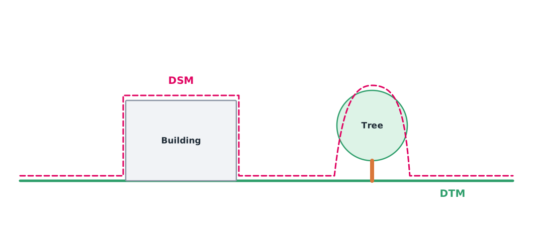
An RGB camera only sees what reflected light reaches, so under dense vegetation there may be no image of the ground at all. LiDAR measures distance from the travel time of laser light and may obtain ground points through gaps in the canopy, but it needs good calibration and navigation. The USGS sets requirements for LiDAR data in its Lidar Base Specification. Point cloud files from the two methods may look alike, but their evidence and limits differ.
Stockpile volume
Volume is computed from a height grid: each cell has area and a height equal to the surface minus the base. The result depends heavily on the chosen base level, and cells with no data must be reported, not counted as zero.
Example 2. Volume from a DSM grid and the effect of the base level
CELL_AREA = 2.0 * 2.0          # m² per cell
dsm = [  # surface height (m), None = no data
    [100.0, 101.0, 102.0, 100.0],
    [101.0, 103.0, 104.0, 101.0],
    [100.0, 102.0, None, 100.0],
]

def volume(base_level):
    cells = [z for row in dsm for z in row if z is not None]
    return sum(CELL_AREA * max(z - base_level, 0.0) for z in cells)

missing = sum(z is None for row in dsm for z in row)
for base in (100.0, 100.5):
    print(f"base {base} m: volume {volume(base):.0f} m3")
print(f"cells without data: {missing} of {sum(len(r) for r in dsm)} -> report, do not treat as zero")
base 100.0 m: volume 56 m3
base 100.5 m: volume 42 m3
cells without data: 1 of 12 -> report, do not treat as zeroRaising the base by only 0.5 m reduces the volume by a quarter, so the base level must be agreed with the user and recorded in the report. The cell with no data lies in the middle of the pile; counting it as zero would understate the volume. Collect more images, or state how the value was estimated.
Module lab
Lab: processing the first image set
- Process the images from modules 1–2 in WebODM or the software set by the lab, using the GCPs for adjustment and keeping the checkpoints aside
- Read the processing report and record the number of images aligned, the number of tie points and the reprojection error; explain which of these cannot show accuracy
- Open the orthomosaic, DSM and point cloud in QGIS, find distorted areas or holes, and trace their causes in the original images
- Agree the stockpile base level with the “user” (the instructor), compute the volume in QGIS and with Example 2, and compare
- Make a table of deliverables stating which question each file answers and what it still cannot answer
Common mistakes
Watch out
- Treating reprojection error as map accuracy
- Calling a DSM a DTM to make the delivery look complete
- Counting no-data cells as zero height in a volume calculation
- Not recording the base level used for the volume
- Exporting a raster at a smaller pixel size and believing detail has been added
Summary
- Depth comes from parallax when the camera moves; heights are sensitive to parallax error
- SfM estimates cameras and shape together; bundle adjustment minimises reprojection differences, and reprojection error is internal consistency
- Choose outputs to match the question: the DSM is the top surface, the DTM is the ground
- Volume depends on the base level, and areas without data must be disclosed
Check your understanding
- = 20 m, = 8.8 mm and the parallax is 2.2 mm. What is the depth?
- A reprojection error of 0.8 pixels means the map is within 0.8 pixels on the ground. True or false?
- A user wants to design drainage in an area with trees. Should they use the DSM or the DTM, and what should they watch for?
- A grid of 5 cells, each 4 m², is 1, 1, 2, 2 and 3 m above the base. What is the volume?
- Why must no-data cells not be counted as zero?
Answers
- m
- False. It is internal consistency on the images; accuracy must be measured at checkpoints
- The DTM, after checking that there really is ground data under the trees rather than an estimate from the canopy edge
- m³
- It understates the volume; the gap must be reported and either filled with more data or its estimation method stated
Key formulas
| Depth from parallax (parallel image pair) | |
| Sensitivity of depth to parallax | |
| Volume from a grid |
Key references
- Wolf, P. R., DeWitt, B. A., & Wilkinson, B. E. (2014). Elements of photogrammetry with applications in GIS (4th ed.). McGraw-Hill Education. link
- Snavely, N., Seitz, S. M., & Szeliski, R. (2006). Photo tourism: Exploring photo collections in 3D. ACM Transactions on Graphics, 25(3), 835–846. link
- Westoby, M. J., Brasington, J., Glasser, N. F., Hambrey, M. J., & Reynolds, J. M. (2012). 'Structure-from-Motion' photogrammetry: A low-cost, effective tool for geoscience applications. Geomorphology, 179, 300–314. link
- Mapillary. Incremental reconstruction algorithm. OpenSfM documentation. link
- OpenDroneMap Authors. Outputs. OpenDroneMap documentation (Version 3.5). link
- U.S. Geological Survey. (2025). Lidar base specification (2025 rev. A). link
- Sampath, A., Shrestha, M., While, M., & Scholl, V. M. (2023). Guidelines for calibration of uncrewed aircraft systems imagery (Open-File Report 2023–1033). U.S. Geological Survey. link
Further reading
Study the assigned knowledge units in advance, review media and take the module quiz
In class / field
Intensive lab and field practice recorded in a lab notebook
Learning evidence: Lab notebook signed by the instructor