Anomaly analysis
UAT 362 Unmanned Aircraft Systems Technology for Industrial, Energy and Infrastructure Applications
Lesson
By the end of this module you will be able to
- Read a confusion matrix and compute precision, recall and F1 for an anomaly detection system
- Choose a model threshold according to the cost of misses versus false alarms
- Compute a frame sampling rate from video so images overlap enough for analysis
- Explain the limits of RGB and thermal images before drawing conclusions
Why this matters
One solar farm inspection yields thousands of images or hours of video, far too many for people to view. AI can shortlist suspicious images, but every AI both misses and raises false alarms. The key question is not “is the AI accurate?” but “how many defects does it miss, how many false alarms does it raise, and what can we accept?”, which depends on how much more expensive one missed defect is than sending someone to check a spot with nothing wrong.
The confusion matrix
Comparing AI results with specialists’ confirmation gives four groups:
- TP (true positive): AI says defect, and it is a defect
- FP (false positive): AI says defect, but it is normal, a false alarm
- FN (false negative): AI says normal, but it is a defect, a miss
- TN (true negative): AI says normal, and it is normal
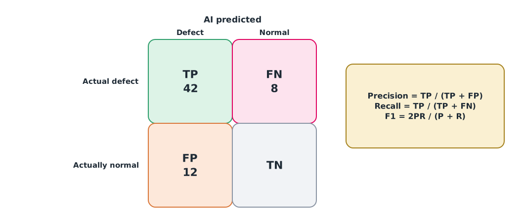
Following the definitions in the scikit-learn documentation, precision is the share of alarms that are correct, recall is the share of real defects that are found, and F1 is their harmonic mean. In asset inspection TN is usually huge, so accuracy always looks high and is of little use.
Example 1. Choosing a threshold from precision and recall
The test set has 50 real defects confirmed by specialists. The detector gives each candidate a confidence score.
results = {  # threshold: (TP, FP, FN)
    0.3: (46, 30, 4),
    0.5: (42, 12, 8),
    0.7: (33, 4, 17),
}
for th, (tp, fp, fn) in results.items():
    p, r = tp / (tp + fp), tp / (tp + fn)
    f1 = 2 * p * r / (p + r)
    print(f"threshold {th}: precision {p:.3f}, recall {r:.3f}, F1 {f1:.3f}, "
          f"missed {fn}, false alarms {fp}")
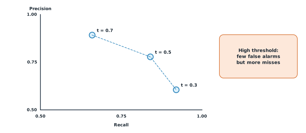
threshold 0.3: precision 0.605, recall 0.920, F1 0.730, missed 4, false alarms 30
threshold 0.5: precision 0.778, recall 0.840, F1 0.808, missed 8, false alarms 12
threshold 0.7: precision 0.892, recall 0.660, F1 0.759, missed 17, false alarms 4Threshold 0.5 gives the highest F1, but that is not necessarily the best choice. If missing one hot joint could black out the whole estate, the team might choose 0.3, which misses only 4, and have people screen out the 30 false alarms. Choosing a threshold is a business and safety decision, not just a statistic.
From video to analysable images
A 30 frames-per-second video contains many repeated images. Analysing every frame wastes time and counts one defect many times, so frames should be sampled to give just the overlap needed.
Example 2. Sampling frames from video
One frame covers 20 m of ground along track, 80% overlap is required, the flight speed is 5 m/s and the video is 30 fps.
FOOT_ALONG, OVERLAP, SPEED, FPS = 20.0, 0.80, 5.0, 30

interval_s = FOOT_ALONG * (1 - OVERLAP) / SPEED
step = int(interval_s * FPS + 1e-9)
print(f"need one frame every {interval_s:.2f} s = one in every {step} frames at {FPS} fps")
print(f"a 10-minute video: {10 * 60 * FPS:,} frames -> {10 * 60 * FPS // step:,} frames to analyse")
need one frame every 0.80 s = one in every 24 frames at 30 fps
a 10-minute video: 18,000 frames -> 750 frames to analyseSampling cuts the work by a factor of tens, but blur must still be checked (module 1), because video often uses slower shutters than still images, and detections repeated across frames must be merged into one location.
Image limits
The knowledge unit on the limits of RGB and thermal images warns that colour on an image is not a measurement: a thermal image exported as colour without radiometric data cannot be read as temperature. Something hidden does not appear in the image, but that does not mean it is absent, and comparing two images with different palettes or scales cannot show a trend. Reports must therefore separate “what is seen”, “what is hidden” and “what is still unknown”.
Module lab
Lab: evaluating an anomaly detection model
- Prepare a test image set labelled by specialists, separate from the set used to train the model
- Run a detector (for example from UAT 322) and record TP, FP and FN at no fewer than three thresholds
- Use Example 1 to compute precision, recall and F1, and choose a threshold with reasons based on cost and safety
- Sample frames from a real video with Example 2 and check that there are no gaps
- Write a report separating what is seen, what is hidden and what is still unknown
Common mistakes
Watch out
- Reporting accuracy when normal images vastly outnumber defects
- Testing on the same images used for training
- Choosing the threshold from F1 alone without considering the cost of misses
- Counting one defect many times from several frames
- Reading temperature from the colours of a thermal image without measurement data
Summary
- The confusion matrix separates TP, FP, FN and TN; precision measures correct alarms and recall measures defects found
- The threshold trades precision against recall and must be chosen by the cost of misses and false alarms
- Sample video frames for the required overlap and merge repeated detections
- Colour is not a measurement, and hidden does not mean absent
Check your understanding
- TP = 30, FP = 10 and FN = 20. What are precision and recall?
- Using question 1, what is F1?
- If missing a defect is very costly, should the threshold be high or low?
- With a 15 m footprint, 75% overlap, 5 m/s and 30 fps video, how often must a frame be used?
- Why is accuracy misleading in asset inspection?
Answers
- ,
- Low, for high recall, with people screening out false alarms
- s, so about one in every frames
- Normal images are so numerous that a model answering “normal” every time still scores high accuracy
Key formulas
| Precision and recall | |
| F1 | |
| Interval between frames used |
Key references
- scikit-learn developers. Metrics and scoring: Quantifying the quality of predictions (scikit-learn 1.9). link
- Szeliski, R. (2022). Computer vision: Algorithms and applications (2nd ed.). Springer. link
- OpenCV. OpenCV documentation. link
- Redmon, J., Divvala, S., Girshick, R., & Farhadi, A. (2016). You only look once: Unified, real-time object detection. In Proceedings of CVPR 2016 (pp. 779–788). link
- Memari, M., Shakya, P., Shekaramiz, M., Seibi, A. C., & Masoum, M. A. S. (2024). Review on the advancements in wind turbine blade inspection: Integrating drone and deep learning technologies for enhanced defect detection. IEEE Access, 12, 33236–33282. link
- O'Connor, J., Smith, M. J., & James, M. R. (2017). Cameras and settings for aerial surveys in the geosciences: Optimising image data. Progress in Physical Geography, 41(3), 325–344. link
Further reading
Study the assigned knowledge units in advance, review media and take the module quiz
Intelligent video analytics
Limitations of RGB and thermal imagery
In class / field
Intensive lab and field practice recorded in a lab notebook
Learning evidence: Lab notebook signed by the instructor