Energy systems
UAT 362 Unmanned Aircraft Systems Technology for Industrial, Energy and Infrastructure Applications
Lesson
By the end of this module you will be able to
- Read thermal patterns on solar arrays and separate module-level from string-level anomalies
- Identify inspection methods for power lines, wind turbines and pipelines with suitable sensors
- Plan pipeline patrol frequency by class location
- Explain the scope of standards and what must still be confirmed on the ground
Why this matters
Each energy system fails in its own way. A whole string running warm and a single hot module have different causes, line joints heat up with current, wind turbine blades erode at the leading edge, and gas leaks are invisible to the eye. Reading the pattern correctly sends the repair team to the right place with the right equipment.
Solar farms
Outdoor thermography of PV modules is covered by the technical specification IEC TS 62446-3:2017, which includes clauses on classes of abnormalities and a table of module thermal patterns. The detailed criteria are in the standard itself, which must be obtained for real work. This module practises a principle common to all of them: compare a module with modules of the same type under the same conditions.
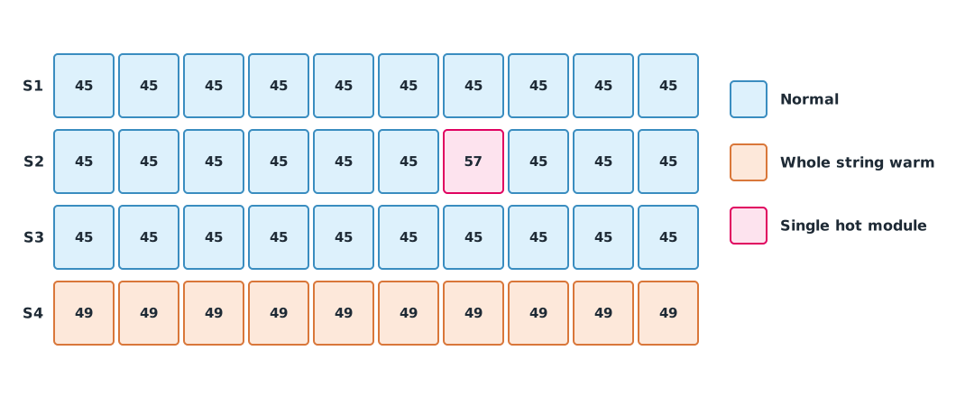
Example 1. Separating string-level from module-level anomalies
Compare at two levels: each string median against the whole array, and each module against its own string median. The 2 K and 5 K criteria are the team’s, for practice.
from statistics import median

temps = [[45.0 + 0.1 * ((i * 7 + j * 3) % 5) for j in range(10)] for i in range(4)]
temps[1][6] += 12.0                     # single hot module
temps[3] = [t + 4.0 for t in temps[3]]  # whole string warm

array_median = median(t for row in temps for t in row)
for s, row in enumerate(temps, 1):
    s_median = median(row)
    string_flag = "string warm" if s_median - array_median >= 2 else ""
    hot = [f"module {m} +{t - s_median:.1f} K" for m, t in enumerate(row, 1) if t - s_median >= 5]
    print(f"S{s}: median {s_median:.2f} °C ({s_median - array_median:+.2f} K) {string_flag} {' '.join(hot)}")
S1: median 45.20 °C (-0.10 K)
S2: median 45.25 °C (-0.05 K) module 7 +11.8 K
S3: median 45.20 °C (-0.10 K)
S4: median 49.20 °C (+3.90 K) string warmS2 has a single abnormally hot module, which must be checked. S4 is warm as a whole with no module standing out within it. This pattern points to a string-level problem, such as a string not delivering current, so the team should check the connections and inverter rather than replace all ten modules. Comparing with the array average alone would miss this difference.
Power lines, wind turbines and pipelines
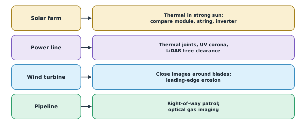
- Power lines: loose or dirty joints have higher resistance and heat up with the current flowing, so inspect at high load and record the current at the time. Corona is inspected with UV cameras (module 2)
- Wind turbines: the review by Memari and colleagues (2024) summarises drone and deep-learning inspection for cracks, leading-edge erosion and delamination of blades. The turbine must be stopped and the rotor locked before flying close
- Gas pipelines: optical gas imaging (OGI) has criteria in EPA 40 CFR 60 Appendix K (2024), such as the camera’s band overlapping an absorption band of the target gas. TDLAS sensors tune a laser across a gas absorption line and compute concentration from the Beer–Lambert law (Lin and colleagues, 2022)
Pipeline patrol frequency
The US rule 49 CFR 192.705 is an example of setting patrol frequency by class location, which depends on the density of buildings near the pipe: the more people, the more frequent the patrols, and road or railway crossings are patrolled more often than elsewhere.
Example 2. Minimum patrols per year (following the US rule as an example)
The assumed 3 km pipeline has a 2.4 km class 1 segment and a 0.6 km class 3 segment with a road crossing.
MIN_PER_YEAR = {  # class location: (at road/rail crossings, elsewhere) minimum per year
    1: (2, 1), 2: (2, 1), 3: (4, 2), 4: (4, 4),
}
segments = [("A", 1, 2.4, False), ("B", 3, 0.6, True)]   # name, class, km, has road crossing
for name, cls, km, crossing in segments:
    crossing_n, elsewhere_n = MIN_PER_YEAR[cls]
    n = max(crossing_n if crossing else 0, elsewhere_n)
    print(f"segment {name}: class {cls}, {km} km -> at least {n} patrols/year")
plan = max(max(MIN_PER_YEAR[c][0] if x else 0, MIN_PER_YEAR[c][1]) for _, c, _, x in segments)
print(f"one patrol plan covering the whole route: {plan} times/year")
segment A: class 1, 2.4 km -> at least 1 patrols/year
segment B: class 3, 0.6 km -> at least 4 patrols/year
one patrol plan covering the whole route: 4 times/yearFlying the whole route in one patrol is simpler than separate schedules per segment, so the frequency of the most demanding segment is used. These numbers are an example from US law; work in Thailand must follow the regulator’s and pipeline owner’s requirements.
Module lab
Lab: reading thermal patterns on a solar array
- Take thermal images of the campus solar array on a sunny day, recording irradiance, air temperature and wind
- Build a table of module temperatures following the real string layout (ask the system operator for it)
- Use Example 1 to separate module-level and string-level anomalies, with criteria set before viewing the results
- Confirm the findings with colour images and inverter current data
- Write a findings list with module positions, possible causes and follow-up checks
Common mistakes
Watch out
- Replacing a whole string of modules when the problem is a connection
- Comparing only with the array average
- Inspecting line joints at low load, so heating does not show
- Flying close to a wind turbine that is still turning
- Quoting IEC abnormality class criteria without having the standard
Summary
- Compare modules with their own group, separating module-level from string-level anomalies, which have different causes
- Inspect power lines at high load together with UV; stop wind turbines before flying close; use OGI or TDLAS for gas pipelines
- Pipeline patrol frequency depends on class location; a single-route plan uses the frequency of the most demanding segment
- Detailed criteria are in the standards and the asset owner’s requirements; drone findings must be confirmed on the ground
Check your understanding
- A string median is 46 °C and one module is 53 °C. What is the difference from the median?
- A whole string runs uniformly warmer than the array. What should be checked first?
- Why should line joints be inspected at high load?
- Under the US rule example, how many times a year must a class 3 segment with a road crossing be patrolled?
- What property must an OGI camera have under Appendix K?
Answers
- K
- The string’s connections and the inverter
- Joint heating increases with current; at low load the anomaly may not show
- 4 times
- Its spectral band must overlap an absorption band of the target gas
Key formulas
| Difference from the group median |
Key references
- International Electrotechnical Commission. (2017). Photovoltaic (PV) systems – Requirements for testing, documentation and maintenance – Part 3: Photovoltaic modules and plants – Outdoor infrared thermography (IEC TS 62446-3:2017). link
- Jahn, U., Herz, M., Köntges, M., et al. (2018). Review on infrared and electroluminescence imaging for PV field applications (Report IEA-PVPS T13-10:2018). IEA PVPS. link
- Memari, M., Shakya, P., Shekaramiz, M., Seibi, A. C., & Masoum, M. A. S. (2024). Review on the advancements in wind turbine blade inspection: Integrating drone and deep learning technologies for enhanced defect detection. IEEE Access, 12, 33236–33282. link
- U.S. Environmental Protection Agency. (2024). Appendix K to Part 60 — Determination of volatile organic compound and greenhouse gas leaks using optical gas imaging. 40 C.F.R. Part 60. link
- Lin, S., Chang, J., Sun, J., & Xu, P. (2022). Improvement of the detection sensitivity for tunable diode laser absorption spectroscopy: A review. Frontiers in Physics, 10, 853966. link
- Transmission lines: Patrolling, 49 C.F.R. § 192.705. link
- Wang, Y., & Qian, Y. (2019). Characteristics of the corona discharge of polymer insulators based on solar-blind ultraviolet images. Optical Engineering, 58(11), 113102. link
Further reading
Study the assigned knowledge units in advance, review media and take the module quiz
In class / field
Intensive lab and field practice recorded in a lab notebook
Learning evidence: Lab notebook signed by the instructor