Multispectral data

Why this matters

The values in a camera image are digital numbers (DN), which depend on the sunlight at the time, the camera settings and the sensitivity of each band. The same rice leaf photographed in bright sun and under cloud gives very different DNs. Compute a vegetation index directly from DN, compare two weeks, and you may conclude the crop got worse when it was only cloudier that day. Calibration converts DN to reflectance, a property of the surface itself, so it can be compared across days and cameras.

Pixel values and reflectance

Reflectance is the fraction of incoming light a surface reflects, from 0 to 1. It is like measuring how white a sheet of paper is, which should not change whether the lights are bright or dim. DN is like the brightness you see in a photo, which does change with the light.

The MicaSense RedEdge-P comes with two items for this:

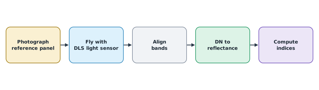
• Calibrated reflectance panel (CRP) with known reflectance in each band, photographed before and after each flight
• Downwelling light sensor (DLS2) on top of the drone, measuring incoming sunlight in each band throughout the flight, used to correct for changing light

The empirical line method

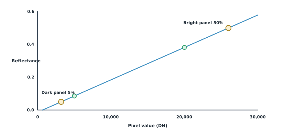
The empirical line method (Smith and Milton, 1999) uses at least two targets of known reflectance, fits a straight line between DN and reflectance, and applies that line to every pixel in the same band. The USGS report (2023) highlights this two-panel method for drone work. It must be done band by band, because each band has a different sensitivity.

PANELS = (0.05, 0.50)                          # reflectance of the dark and bright panels
panel_dn = {"red": (3200, 26000), "nir": (2500, 21000)}
crop_dn = {"red": 5000, "nir": 20000}          # DN of the rice leaf in each band

def calibrate(dn, dn_pair, rho_pair=PANELS):
    gain = (dn_pair[1] - dn_pair[0]) / (rho_pair[1] - rho_pair[0])
    offset = dn_pair[0] - gain * rho_pair[0]
    return (dn - offset) / gain

rho = {band: calibrate(crop_dn[band], panel_dn[band]) for band in crop_dn}
ndvi_rho = (rho["nir"] - rho["red"]) / (rho["nir"] + rho["red"])
ndvi_dn = (crop_dn["nir"] - crop_dn["red"]) / (crop_dn["nir"] + crop_dn["red"])
print(f"reflectance red {rho['red']:.3f}, NIR {rho['nir']:.3f}")
print(f"NDVI from reflectance {ndvi_rho:.3f} vs from raw DN {ndvi_dn:.3f}")

reflectance red 0.086, NIR 0.476
NDVI from reflectance 0.695 vs from raw DN 0.600

Light changing during flight

If the panel is photographed in bright sun but cloud covers part of the field during the flight, those pixels get reflectance that is too low. The DLS measures light at each image, so it can correct by the light ratio. Cloud reduces light by different amounts in each band, so vegetation indices are affected too, not just reflectance.

true_rho = {"red": 0.06, "nir": 0.40}
light_ratio = {"red": 0.70, "nir": 0.80}      # light at image / light at panel

def ndvi(r): return (r["nir"] - r["red"]) / (r["nir"] + r["red"])

raw = {b: true_rho[b] * light_ratio[b] for b in true_rho}      # no light correction
fixed = {b: raw[b] / light_ratio[b] for b in raw}              # corrected with DLS
for name, r in (("true", true_rho), ("no DLS correction", raw), ("with DLS correction", fixed)):
    print(f"{name:<20} red {r['red']:.3f}  NIR {r['nir']:.3f}  NDVI {ndvi(r):.3f}")

true                 red 0.060  NIR 0.400  NDVI 0.739
no DLS correction    red 0.042  NIR 0.320  NDVI 0.768
with DLS correction  red 0.060  NIR 0.400  NDVI 0.739

Band alignment

A multispectral camera uses a separate lens for each band, each looking from a slightly different position. Without band alignment, the same pixel in each band may be a different spot on the ground, and field bunds show false index values along their edges. MicaSense’s imageprocessing code (MIT licence) includes examples of panel calibration and image alignment that can be tried without a camera.

Module lab

Common mistakes

Summary

• DN depends on light and camera; reflectance is a surface property and must be derived before analysis
• The CRP provides the reference; the DLS corrects for light changes during flight
• The empirical line fits a straight line from at least two reference panels, band by band
• Uneven light and misaligned bands produce false index patterns

Check your understanding

1. The 5% panel gives DN 3,200 and the 50% panel DN 26,000. What is the gain of the line?
2. Using question 1, what is the reflectance of a pixel with DN 14,600?
3. A raw reflectance of 0.042 was captured when light was at 70%. What is it after correction?
4. Why must calibration be done band by band?
5. What does skipping band alignment do to an index map?