Vegetation indices and GIS
UAT 365 Unmanned Aircraft Systems Technology for Smart Agriculture and Remote Sensing
Lesson
By the end of this module you will be able to
- Compute and interpret NDVI, NDRE and GNDVI from reflectance
- Divide a field into zones with criteria set in advance, and compute zone areas in rai
- Use QGIS to compute indices from rasters and lay out a zone map the recipient can read unaided
- Explain the limits of vegetation indices and the need for ground truth
Why this matters
Five bands of reflectance for every pixel is a mass of numbers no farmer can act on. A vegetation index combines the plant-related bands into one number per pixel, and zoning turns those numbers into areas you can act on, such as “this 5-rai zone needs a visit”. But without understanding what an index does and does not measure, you might fertilise a spot whose real problem is waterlogging.
Three vegetation indices
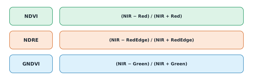
- NDVI (Rouse and colleagues, 1974; Tucker, 1979) uses the contrast between NIR, which leaves reflect strongly, and red, which chlorophyll absorbs. It ranges from −1 to 1: dense healthy vegetation is high, bare soil low and water usually negative
- NDRE (Barnes and colleagues, 2000) uses the red-edge band instead of red. The red edge is sensitive to chlorophyll content in dense canopies, and Barnes and colleagues used it with other indices to monitor crop nitrogen status
- GNDVI (Gitelson and colleagues, 1996) uses the green band instead of red
Because indices are ratios they partly cancel differences in brightness, but they do not replace the calibration of module 2.
Example 1. Three indices for a healthy and a stressed pixel
pixels = {  # reflectance: green, red, red edge, NIR
    "healthy": {"green": 0.08, "red": 0.04, "rededge": 0.20, "nir": 0.50},
    "stressed": {"green": 0.10, "red": 0.09, "rededge": 0.22, "nir": 0.35},
}
nd = lambda a, b: (a - b) / (a + b)
for name, p in pixels.items():
    print(f"{name:<9} NDVI {nd(p['nir'], p['red']):.3f}  NDRE {nd(p['nir'], p['rededge']):.3f}  "
          f"GNDVI {nd(p['nir'], p['green']):.3f}")
healthy NDVI 0.852 NDRE 0.429 GNDVI 0.724
stressed NDVI 0.591 NDRE 0.228 GNDVI 0.556All three indices fall for the stressed pixel, but by different amounts. Each index has its own range, so NDVI thresholds must never be applied to NDRE, and only the same index from the same camera and calibration should be compared.
Zoning the field
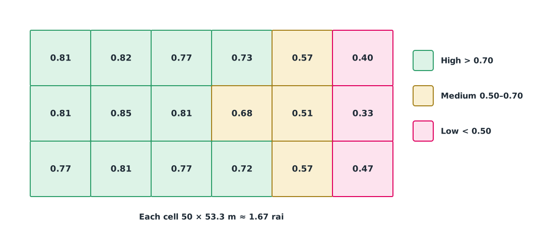
Our rice field is divided into a 3 × 6 grid of cells, each 50 × 53.3 m (about 1.67 rai). In practice each cell would hold the mean of its pixels, and cells are assigned to zones with criteria agreed before seeing the results.
Example 2. NDVI per cell, zones and areas in rai
NIR = [[0.48, 0.50, 0.47, 0.44, 0.36, 0.30], [0.49, 0.51, 0.48, 0.42, 0.34, 0.28], [0.47, 0.49, 0.46, 0.43, 0.37, 0.33]]
RED = [[0.05, 0.05, 0.06, 0.07, 0.10, 0.13], [0.05, 0.04, 0.05, 0.08, 0.11, 0.14], [0.06, 0.05, 0.06, 0.07, 0.10, 0.12]]
CELL_RAI = (300 / 6) * (160 / 3) / 1600

def zone(v): return "high" if v > 0.70 else ("medium" if v >= 0.50 else "low")

counts = {"high": 0, "medium": 0, "low": 0}
for n_row, r_row in zip(NIR, RED):
    values = [(n - r) / (n + r) for n, r in zip(n_row, r_row)]
    print(" ".join(f"{v:.2f}" for v in values))
    for v in values:
        counts[zone(v)] += 1
for z, c in counts.items():
    print(f"{z:<6} {c:>2} cells = {c * CELL_RAI:.2f} rai")
0.81 0.82 0.77 0.73 0.57 0.40
0.81 0.85 0.81 0.68 0.51 0.33
0.77 0.81 0.77 0.72 0.57 0.47
high 11 cells = 18.33 rai
medium 4 cells = 6.67 rai
low 3 cells = 5.00 raiThe low zone runs along the whole right-hand edge of the field. A long, linear pattern like this usually points to a spatial cause, such as the tail end of an irrigation canal, a different soil or different management. Visit the field before concluding it is a nutrient shortage.
Doing it in QGIS
QGIS computes indices from reflectance rasters with the Raster Calculator, for example ("nir@1" - "red@1") / ("nir@1" + "red@1"). Zones are then made by reclassifying value ranges and converting to polygons to compute areas. Use a coordinate system in metres (such as UTM 47N) and divide by 1,600 to get rai. The map layout must show the image date, the index and criteria used, a scale and the ground-truth status (see map layout in UAT 361).
Limits of vegetation indices
- A low index says “something is wrong” but not why: nutrient shortage, water shortage, disease, insects, weeds or simply young plants
- Before the rice canopy closes, pixels mix soil and paddy water, so compare only the same growth stage
- The zone thresholds in this module are assumed for practice; real thresholds must come from local data and agronomists
Module lab
Lab: a field zone map
- Load the reflectance rasters from module 2 into QGIS and compute NDVI and NDRE with the Raster Calculator
- Set zone thresholds before looking at the map and record the reasons, then zone the field and compute areas in rai; compare with Example 2
- Choose at least two ground-truth points per zone, visit them, and photograph and record plant height, leaf colour, water level and any symptoms
- Compare the ground observations with the zones, and state which zones are explained and which still have unknown causes
- Lay out a zone map the farmer can read unaided, and submit it with the zone GeoPackage and the ground-truth record
Common mistakes
Watch out
- Using one index’s thresholds for another
- Setting zone thresholds after seeing the map to get the expected result
- Concluding causes from map colours without visiting the field
- Computing areas in a degree-based coordinate system instead of one in metres
- Comparing maps from different growth stages and concluding the crop is getting worse
Summary
- NDVI uses NIR and red, NDRE NIR and red edge, GNDVI NIR and green; each has its own range
- Zone with thresholds set in advance, then compute areas in rai in a metre-based coordinate system
- Indices show where something is abnormal; ground truth shows why
- Delivered maps must state the date, index, thresholds and verification status
Check your understanding
- NIR = 0.45 and Red = 0.05. What is NDVI?
- NIR = 0.45 and RedEdge = 0.25. What is NDRE?
- A field of 18 cells, each 1.67 rai, has 3 cells in the low zone. How many rai is the low zone?
- Why should a low zone running along one edge of the field be checked for water first?
- Does a low NDVI tell you the cause of the problem?
Answers
- rai
- Spatial patterns usually come from spatial factors such as the end of a watercourse or soil, rather than diseases that appear in patches
- No. It only shows an abnormality; ground truth is needed to find the cause
Key formulas
| NDVI | |
| NDRE | |
| GNDVI |
Key references
- Rouse, J. W., Haas, R. H., Schell, J. A., & Deering, D. W. (1974). Monitoring vegetation systems in the Great Plains with ERTS. Third ERTS-1 Symposium, NASA. link
- Tucker, C. J. (1979). Red and photographic infrared linear combinations for monitoring vegetation. Remote Sensing of Environment, 8(2), 127–150. link
- Barnes, E. M., Clarke, T. R., Richards, S. E., Colaizzi, P. D., Haberland, J., Kostrzewski, M., Waller, P., Choi, C., Riley, E., Thompson, T., Lascano, R. J., Li, H., & Moran, M. S. (2000). Coincident detection of crop water stress, nitrogen status and canopy density using ground-based multispectral data. In Proceedings of the Fifth International Conference on Precision Agriculture. ASA-CSSA-SSSA. link
- Gitelson, A. A., Kaufman, Y. J., & Merzlyak, M. N. (1996). Use of a green channel in remote sensing of global vegetation from EOS-MODIS. Remote Sensing of Environment, 58(3), 289–298. link
- QGIS Project. QGIS user guide. link
- Lillesand, T., Kiefer, R. W., & Chipman, J. (2015). Remote sensing and image interpretation (7th ed.). Wiley. link
Further reading
Study the assigned knowledge units in advance, review media and take the module quiz
In class / field
Intensive lab and field practice recorded in a lab notebook
Learning evidence: Lab notebook signed by the instructor