Spatial decision-making
UAT 365 Unmanned Aircraft Systems Technology for Smart Agriculture and Remote Sensing
Lesson
By the end of this module you will be able to
- Compute the crop water stress index (CWSI) from canopy temperature
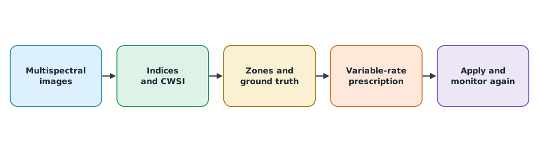
- Combine vegetation index zones, CWSI and ground truth into a variable-rate prescription map
- Separate real change from uncertainty with the LoD95 detection level
- Pass results into a decision support system together with their limits
Why this matters
A beautiful vegetation index map is not yet an answer. The farmer wants to know what to do, where, how much, and whether it worked. This module turns the data from earlier modules into decisions and follows them up honestly. The example shows that looking at the vegetation index alone and fertilising the low zone may treat the wrong problem, because the real cause is water stress.
Water stress
When a plant has enough water, its leaves transpire and cool down, like sweat evaporating from skin. When it is short of water, the stomata close and the leaves warm up. The crop water stress index (CWSI), developed by Idso and colleagues and Jackson and colleagues (1981), compares canopy temperature with two reference temperatures:
is the temperature of a fully transpiring leaf and that of a non-transpiring leaf. Maes and Steppe (2012) summarise that a CWSI of 0 means no stress and 1 means fully closed stomata. Both references come from wet and dry reference targets in the field or from a model and depend on the weather at the time, so they must be measured on the same day.
From zones to a prescription map
A prescription map tells the sprayer what rate to apply in each zone. The decision must combine several kinds of evidence, not a single index.
Example 1. Combining NDVI and CWSI before issuing a prescription
Zone areas come from module 3. Canopy and reference temperatures are assumed, and the liquid fertiliser rate per zone is assumed to be set by an agronomist.
T_WET, T_DRY = 26.0, 36.0                     # °C from reference targets on the same day
zones = {  # zone: (area rai, canopy temperature °C, prescribed liquid fertiliser L/ha)
    "high": (18.33, 28.5, 10.0),
    "medium": (6.67, 31.0, 15.0),
    "low": (5.00, 34.0, 20.0),
}
total = 0.0
for name, (rai, canopy, rate) in zones.items():
    cwsi = (canopy - T_WET) / (T_DRY - T_WET)
    if cwsi >= 0.6:
        action, rate = "check irrigation first, hold fertiliser", 0.0
    else:
        action = f"apply {rate:.0f} L/ha"
    litres = rate * rai * 0.16
    total += litres
    print(f"{name:<6} {rai:5.2f} rai  CWSI {cwsi:.2f}  -> {action} ({litres:.1f} L)")
print(f"total product {total:.1f} L")
high 18.33 rai CWSI 0.25 -> apply 10 L/ha (29.3 L)
medium 6.67 rai CWSI 0.50 -> apply 15 L/ha (16.0 L)
low 5.00 rai CWSI 0.80 -> check irrigation first, hold fertiliser (0.0 L)
total product 45.3 LThe low zone has a high CWSI, showing the crop is short of water. More fertiliser there would not fix the problem, so the irrigation must be checked first. The CWSI threshold of 0.6 is assumed for this lesson; real thresholds must come from agronomists and local data (1 rai = 0.16 ha).
Monitoring again: real change or just error?
Two weeks after application, fly again and compare NDVI for each zone. A difference may come from measurement uncertainty (light, calibration, alignment) rather than a change in the crop. Following NIST’s propagation of uncertainty, if the errors of the two surveys are independent:
A difference within the LoD95 must be reported as “not detectable”, not “no change”.
Example 2. Separating detectable change
Assume the NDVI uncertainty of each survey is 0.03 (estimated from reference areas that did not change).
import math

SIGMA_1, SIGMA_2 = 0.03, 0.03
lod = 1.96 * math.hypot(SIGMA_1, SIGMA_2)
change = {"Z1": 0.02, "Z2": -0.05, "Z3": -0.12, "Z4": 0.10}   # NDVI survey 2 − survey 1
print(f"LoD95 = {lod:.3f}")
for zone, d in change.items():
    verdict = ("detected increase" if d > lod else "detected decrease" if d < -lod
               else "not detectable")
    print(f"{zone}: dNDVI {d:+.2f} -> {verdict}")
LoD95 = 0.083
Z1: dNDVI +0.02 -> not detectable
Z2: dNDVI -0.05 -> not detectable
Z3: dNDVI -0.12 -> detected decrease
Z4: dNDVI +0.10 -> detected increase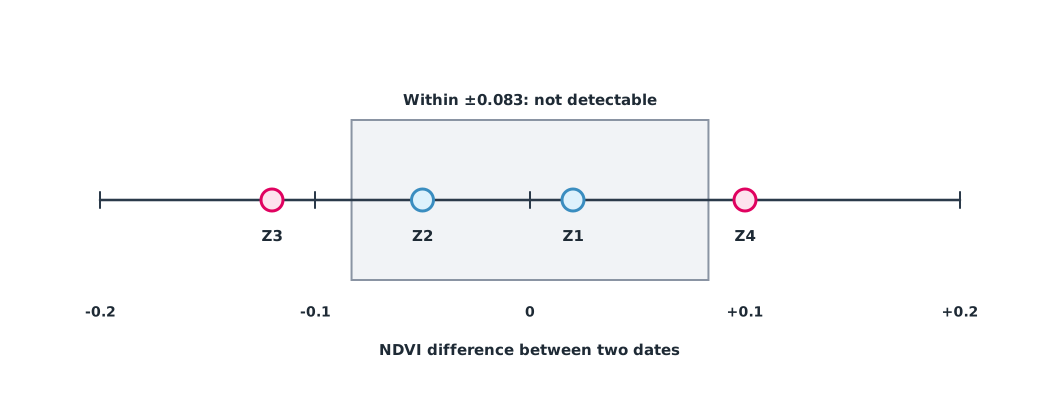
This formula applies when the two errors are independent, unbiased and approximately normal. Otherwise use a method suited to the data. When many pixels are tested at once, some will be “detected” by chance.
Into a decision support system
Results passed into a decision support system or cooperative platform need more than a map: the image dates, camera and calibration method, indices and thresholds, ground-truth results, a recommendation per zone with reasons, and limits such as zones whose cause is still unknown. Deliver GIS layers (such as a GeoPackage) that other systems can read, plus a PDF map for the farmer. The final decision belongs to the farmer and specialists; drone data is supporting evidence.
Module lab
Lab: prescription map and follow-up
- Capture thermal images of the training field with wet and dry reference targets, and compute CWSI per zone
- Combine the NDVI zones from module 3 with CWSI and ground truth, and write the reasoning for each zone’s decision
- Build the prescription map in QGIS and compute the total product with Example 1
- Fly again after treatment, estimate uncertainty from reference areas, and use Example 2 to classify zones as detected or not detectable
- Deliver the data set and a one-page report to the “farmer” (the instructor), with clearly stated limits
Common mistakes
Watch out
- Adding fertiliser to every low-index zone without checking water and other causes
- Using T_wet and T_dry from different days
- Reporting a difference within the LoD as “no change”
- Setting σ low to make change easier to detect
- Delivering only a map without methods, thresholds and limits
Summary
- CWSI = (Tc − Twet)/(Tdry − Twet) indicates water stress: 0 is no stress, 1 is full stress
- A prescription map must combine vegetation indices, CWSI and ground truth, not a single index
- A difference must exceed LoD95 to count as detected change
- Pass results into decision support with methods, thresholds and limits
Check your understanding
- Tc = 30 °C, Twet = 25 °C and Tdry = 35 °C. What is the CWSI?
- σ₁ = 0.02 and σ₂ = 0.04 (independent). What is LoD95?
- Using question 2, is an NDVI difference of −0.07 a detected change?
- How many litres does a 5-rai zone need at 20 L/ha?
- Why should a zone with low NDVI and high CWSI not simply receive more fertiliser?
Answers
- No, because ; report it as not detectable
- L
- The main cause is probably water shortage, which fertiliser does not fix; check the irrigation first
Key formulas
| Crop water stress index | |
| Uncertainty of a difference (independent) | |
| Level of detection |
Key references
- Idso, S. B., Jackson, R. D., Pinter, P. J., Jr., Reginato, R. J., & Hatfield, J. L. (1981). Normalizing the stress-degree-day parameter for environmental variability. Agricultural Meteorology, 24, 45–55. link
- Jackson, R. D., Idso, S. B., Reginato, R. J., & Pinter, P. J., Jr. (1981). Canopy temperature as a crop water stress indicator. Water Resources Research, 17(4), 1133–1138. link
- Maes, W. H., & Steppe, K. (2012). Estimating evapotranspiration and drought stress with ground-based thermal remote sensing in agriculture: A review. Journal of Experimental Botany, 63(13), 4671–4712. link
- NIST/SEMATECH. Propagation of error considerations (section 2.5.5). e-Handbook of statistical methods. link
- International Society of Precision Agriculture. (2024). Precision agriculture definition. link
- QGIS Project. QGIS user guide. link
Further reading
Study the assigned knowledge units in advance, review media and take the module quiz
In class / field
Intensive lab and field practice recorded in a lab notebook
Learning evidence: Lab notebook signed by the instructor