SORA and the Specific category
UAT 401 UAS Regulations, Safety and Risk Management
Lesson
By the end of this module you will be able to
- Define flight geography, contingency volume, operational volume and ground risk buffer under SORA 2.5
- Compute the area used for ground risk assessment from speed, reaction time and height
- Find the maximum population density in the footprint and choose the iGRC table row
- Compare the effect of mitigations with redesigning the area on SAIL
Why this matters
UAT 312 walked through the ten steps of SORA 2.5 and read the tables for iGRC and SAIL in a training case. The drone knowledge base’s unit on the SORA method explains ConOps, GRC, ARC, SAIL and OSOs, and its unit on BVLOS and risk assessment urges linking risks, mitigations and evidence. In real work, the values fed into the tables, such as population density, depend on areas we draw ourselves. This module practises computing those areas and shows that redesigning an area can sometimes achieve as much as adding equipment.
Volumes and buffers in SORA 2.5
SORA 2.5 (JARUS, 2024) defines them as follows. Flight geography is where the drone operates under normal conditions, including margins for system and operational errors. The contingency volume surrounds the flight geography; entering it is an abnormal situation that triggers contingency procedures. The operational volume is the flight geography plus the contingency volume and is the basis for the air risk assessment. The ground risk buffer is the ground area surrounding the contingency volume’s footprint. The main body says the initial buffer could be defined with a 1-to-1 principle (as wide as the flight height) or another value justified under Annex E, and the final buffer is set in Step 8, where it may change with the containment level or mitigations such as a parachute.
Example 1 A suburban survey area next to a village
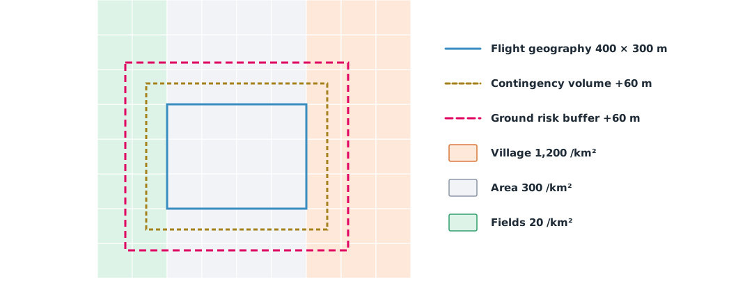
The flight geography is 400 × 300 m, with a maximum height of 60 m, a speed of 15 m/s, a 3 s pilot reaction time and an assumed stopping distance of 15 m. Population data is on a 100 m grid: rice fields to the west at 20 people/km², general area at 300 people/km², and a village to the east at 1,200 people/km² (hypothetical data).
import numpy as np

fg_w, fg_h = 400.0, 300.0     # flight geography (m)
height = 60.0                 # maximum height AGL (m)
speed, react = 15.0, 3.0      # speed m/s and pilot reaction time s
contingency = speed * react + 15.0   # distance during reaction + stopping distance (assumed)
buffer = height               # initial ground risk buffer by the 1-to-1 principle

def area(margin):
    return (fg_w + 2 * margin) * (fg_h + 2 * margin) / 1e6   # km²

print(f"contingency volume width {contingency:.0f} m, ground risk buffer {buffer:.0f} m")
print(f"flight geography {area(0):.3f} km², operational volume {area(contingency):.3f} km², "
      f"with buffer {area(contingency + buffer):.3f} km²")

# population density (people/km²) on a 100 m grid around the area (hypothetical)
x = np.arange(-200, 700, 100) + 50
y = np.arange(-200, 600, 100) + 50
X, Y = np.meshgrid(x, y)
dens = np.where(X >= 450, 1200, 300)         # village to the east
dens = np.where(X < 0, 20, dens)             # rice fields to the west
m = contingency + buffer
cover = (X > -m) & (X < fg_w + m) & (Y > -m) & (Y < fg_h + m)
fg = (X > 0) & (X < fg_w) & (Y > 0) & (Y < fg_h)
print(f"max density in flight geography {dens[fg].max()} /km², "
      f"in footprint with buffer {dens[cover].max()} /km²")
contingency volume width 60 m, ground risk buffer 60 m
flight geography 0.120 km², operational volume 0.218 km², with buffer 0.346 km²
max density in flight geography 300 /km², in footprint with buffer 1200 /km²The area used for ground risk assessment is almost three times the flight geography, and although the route never enters the village, the buffer reaches the village cells. The maximum density to use is therefore 1,200, not 300 people/km². The contingency-width formula in this example is simplified for teaching; real work must include navigation error, wind and the aircraft’s actual stopping performance.
From iGRC to SAIL
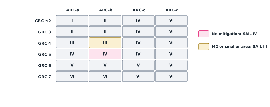
Table 2 of SORA 2.5 gives the iGRC from the aircraft’s maximum size and speed and the population density. For the column up to 1 m and 25 m/s, the density rows below 5, 50, 500, 5,000 and 50,000 people/km² give iGRC 2, 3, 4, 5 and 6, and a controlled ground area gives 1. Table 5 gives ground risk mitigations; for example, M2 (reducing impact energy, such as with a parachute) reduces by 1 at medium robustness and 2 at high. Table 7 converts the final GRC and residual ARC into a SAIL.
Example 2 Add a parachute, or shrink the flight area?
The drone is up to 1 m in size and flies no faster than 25 m/s, with residual ARC-b assumed in all cases. Compare three options: no mitigation; M2 at medium robustness with full evidence; and moving the eastern edge of the flight area 100 m west so the footprint no longer reaches the village (training case).
ROWS = [5, 50, 500, 5000, 50000]            # upper bounds of density rows (people/km²), SORA 2.5 Table 2
IGRC_1M = [2, 3, 4, 5, 6]                    # column 1 m / 25 m/s
MIN_1M = 1                                   # controlled ground area row
SAIL = {2: "I II IV VI", 3: "II II IV VI", 4: "III III IV VI",
        5: "IV IV IV VI", 6: "V V V VI", 7: "VI VI VI VI"}   # Table 7, ARC a b c d

def igrc(density):
    for top, g in zip(ROWS, IGRC_1M):
        if density < top:
            return g
    return 7

def sail(grc, arc):
    return SAIL[max(grc, 2)].split()["abcd".index(arc)]

cases = {
    "village east, no mitigation": (1200, 0, "b"),
    "village east, M2 medium (-1)": (1200, -1, "b"),
    "flight area cut by 100 m": (300, 0, "b"),
}
for name, (d, mit, arc) in cases.items():
    g0 = igrc(d)
    g = max(g0 + mit, MIN_1M)
    print(f"{name:30s} density {d:>5}  iGRC {g0}  final GRC {g}  ARC-{arc}  SAIL {sail(g, arc)}")
village east, no mitigation density 1200 iGRC 5 final GRC 5 ARC-b SAIL IV
village east, M2 medium (-1) density 1200 iGRC 5 final GRC 4 ARC-b SAIL III
flight area cut by 100 m density 300 iGRC 4 final GRC 4 ARC-b SAIL IIIBoth a parachute proven at medium robustness and shrinking the flight area reduce SAIL from IV to III, but at different costs: the parachute needs test evidence under Annex B, while shrinking the area may need an extra flight to cover the remainder. This example is for practice only; real work needs real population data, a real ARC assessment and acceptance by the authority.
Class activity
Activity: designing the area to reduce risk
- Choose a real survey area around the university and draw the flight geography on a map
- Estimate the training drone’s speed, reaction time and stopping distance, and compute the contingency volume and buffer with Example 1
- Find population density from open sources, stating source and year, and find the maximum in the footprint
- Read the tables for SAIL and propose two options that reduce it, with the evidence each needs
- Discuss which values are assumptions and how you would verify them before a real application
Common mistakes
Watch out
- Using density only inside the flight geography, forgetting the buffer
- Setting a contingency volume narrower than the drone’s real stopping distance
- Claiming M2 without evidence at the claimed robustness
- Reducing GRC below the column minimum
- Using training-case values in a real application
Summary
- Operational volume = flight geography + contingency volume, and the buffer surrounds the contingency volume’s footprint
- The initial buffer may use the 1-to-1 principle and is adjusted in Step 8
- Population density must use the maximum over the whole footprint
- Redesigning the area can reduce SAIL as much as adding mitigations
Check your understanding
- How does the contingency volume differ from the flight geography?
- Flying at 80 m with the 1-to-1 principle, how wide is the initial buffer?
- At 12 m/s, 2 s reaction time and 10 m stopping distance, what is the simplified contingency width?
- A 1 m column drone with maximum density 1,200 people/km² has what iGRC?
- Final GRC 4 with residual ARC-c gives what SAIL?
Answers
- Flight geography is the normal operating area; the contingency volume surrounds it, and entering it is an abnormal situation
- 80 m
- m
- 5 (the below-5,000 row)
- SAIL IV
Key formulas
| Contingency volume width (simplified) | |
| Ground risk buffer by the 1-to-1 principle | |
| Final GRC |
Key references
- Joint Authorities for Rulemaking on Unmanned Systems. (2024). JARUS guidelines on Specific Operations Risk Assessment (SORA), main body, edition 2.5 (JAR-DEL-SRM-SORA-MB-2.5). link
- สำนักงานการบินพลเรือนแห่งประเทศไทย. (2569). ประกาศ กพท. เรื่อง หลักเกณฑ์และวิธีการในการอนุญาตให้ผู้บังคับหรือปล่อยอากาศยานซึ่งไม่มีนักบิน ประเภทอากาศยานที่ควบคุมการบินจากภายนอก ที่มีน้ำหนักไม่เกิน 25 กิโลกรัม ปฏิบัติแตกต่างไปจากเงื่อนไขที่กำหนด พ.ศ. 2569 (มีผล 17 พฤษภาคม 2569). link
- International Civil Aviation Organization. (2015). Manual on remotely piloted aircraft systems (RPAS) (Doc 10019). ICAO. link
- European Commission. (2019). Commission Implementing Regulation (EU) 2019/947 on the rules and procedures for the operation of unmanned aircraft. link
Further reading
Study the assigned knowledge units in advance, review media and take the module quiz
In class / field
Lecture, case discussion and in-class problem solving
Learning evidence: Quiz results and submitted exercises