Measurement principles and uncertainty
UAT 205 Sensors and Instrumentation Systems
Lesson
By the end of this module you will be able to
- Explain the measurement chain and sensor characteristics such as range, resolution, sensitivity and nonlinearity
- Build a calibration curve by least squares and compare it with two-point calibration
- Evaluate combined uncertainty with the law of propagation and sensitivity coefficients
- Compute ADC resolution and predict the apparent frequency when aliasing occurs
Why this matters
A drone knows everything about itself through sensors. If a sensor reads slightly wrong, the controller decides on wrong numbers, and the result is a drone that will not hold still, an altitude that drifts, or survey data that cannot be used. This course teaches how each type of sensor measures, how it can be wrong, and how to calibrate it.
The whole course uses one hypothetical case: a lab building a fixed-wing VTOL drone to survey farm plots, which must calibrate its whole sensor set before mission flights. All numbers are made up for practice unless a source is given. The Python code for every module can be downloaded from /downloads/uat-205/.
The measurement chain
A single measurement passes through several stages. The sensor converts a physical quantity, such as temperature or pressure, into an electrical signal. Signal conditioning amplifies and filters it, the ADC converts it to a number, and software applies calibration to convert it back into the desired unit. Every stage can add error, so a complete measurement result always has both a value and an uncertainty (Fraden, 2016).
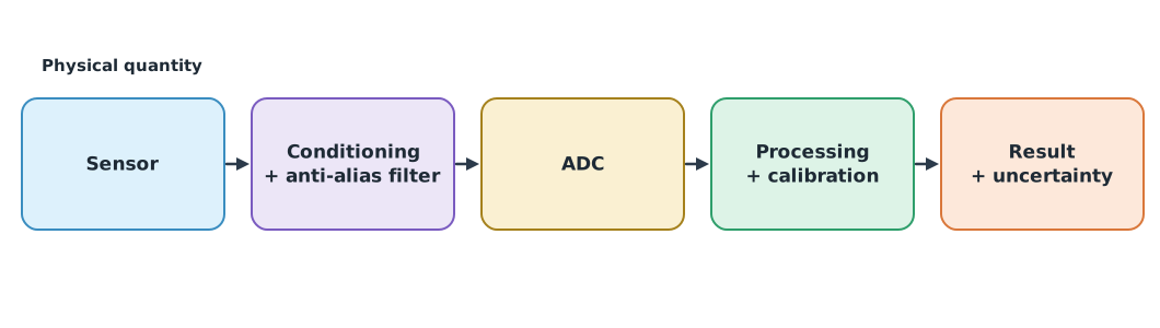
Characteristics to read from the datasheet before choosing a sensor:
- Range: the lowest to highest measurable value; the top of the range is full scale (FS).
- Resolution: the smallest change the system can distinguish, which is not the same as accuracy.
- Sensitivity: output change per unit input, such as mV/°C.
- Nonlinearity: deviation from the straight line used to represent the sensor, often given as %FS.
- Bandwidth and response time: how quickly the sensor follows changes.
The calibration curve
Calibration compares sensor readings with reference values of known uncertainty, then finds the relationship used to correct readings. The simplest method is two-point, using the two end points. Least squares uses every point to find the line with the smallest sum of squared errors, as described in the NIST statistics handbook.
Once the equation is found, the uncertainty of the result is needed. The GUM (JCGM 100:2008), clause 5.1.2, gives the law of propagation of uncertainty: if and the inputs are uncorrelated, the combined uncertainty is , where is the sensitivity coefficient, telling how strongly that input affects the result.
Example 1 Calibrating a battery temperature sensor
The sensor is immersed alongside a reference thermometer (standard uncertainty 0.10 °C) at six temperatures. The multimeter reads voltage with a standard uncertainty of 2 mV.
import math
import statistics as st

T_REF = [0, 10, 20, 30, 40, 50]                   # °C from the reference thermometer
V = [0.502, 0.598, 0.701, 0.797, 0.905, 1.001]     # V from the sensor
FS = 50.0                                          # °C full scale
U_V, U_REF = 0.002, 0.10                           # V, °C standard uncertainties

two_point = ((V[-1] - V[0]) / (T_REF[-1] - T_REF[0]), V[0])
mt, mv = st.mean(T_REF), st.mean(V)
gain = sum((t - mt) * (v - mv) for t, v in zip(T_REF, V)) / sum((t - mt) ** 2 for t in T_REF)
least = (gain, mv - gain * mt)

for name, (a, b) in (("two-point", two_point), ("least squares", least)):
    res = [(v - b) / a - t for t, v in zip(T_REF, V)]
    print(f"{name:<14} {a * 1000:.3f} mV/°C, offset {b:.4f} V, residuals "
          + " ".join(f"{r:+.2f}" for r in res) + f" °C, worst {max(map(abs, res)) / FS:.2%} FS")

a, b = least
res = [(v - b) / a - t for t, v in zip(T_REF, V)]
u_fit = math.sqrt(sum(r * r for r in res) / (len(res) - 2))
c_v = 1 / a                                        # °C per V (sensitivity coefficient)
u_c = math.sqrt((c_v * U_V) ** 2 + U_REF ** 2 + u_fit ** 2)
print(f"c_V = {c_v:.1f} °C/V, u from voltage {c_v * U_V:.2f} °C, u_fit {u_fit:.2f} °C")
print(f"combined u_c = {u_c:.2f} °C, expanded U = {2 * u_c:.2f} °C (k = 2)")
two-point 9.980 mV/°C, offset 0.5020 V, residuals +0.00 -0.38 -0.06 -0.44 +0.38 +0.00 °C, worst 0.88% FS
least squares 10.034 mV/°C, offset 0.4998 V, residuals +0.22 -0.21 +0.05 -0.38 +0.38 -0.05 °C, worst 0.76% FS
c_V = 99.7 °C/V, u from voltage 0.20 °C, u_fit 0.31 °C
combined u_c = 0.38 °C, expanded U = 0.77 °C (k = 2)The least-squares line spreads the error across all points, so its worst error is lower than two-point calibration. The combined uncertainty comes from three sources: the multimeter, magnified by ; the reference thermometer; and the nonlinearity the straight line cannot explain. The largest source is the nonlinearity; to improve the result, reduce it first, for example by fitting a quadratic instead of a line.
ADC and sampling
An -bit ADC with reference voltage divides the range into levels; one level is one LSB. Analog Devices tutorial MT-001 shows that ideal quantization noise has an rms value of , and the ideal SNR for a full-scale sine wave is dB.
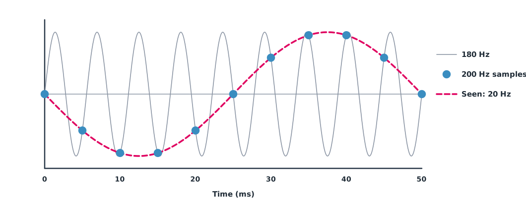
The other key issue is the sampling rate. Following Shannon (1949), you must sample faster than twice the highest frequency in the signal. Otherwise high frequencies disguise themselves as low frequencies that are not really there, which is called aliasing, like car wheels in a video that seem to turn slowly or backwards. On a drone, propeller vibration sampled too slowly can become a slow oscillation that the controller tries to correct. Signal conditioning therefore needs an anti-aliasing filter before the ADC.
Example 2 ADC resolution and alias frequencies
import math

N, VREF = 12, 3.3
lsb = VREF / 2 ** N
print(f"LSB {lsb * 1000:.3f} mV, quantization noise {lsb / math.sqrt(12) * 1000:.3f} mV rms, "
      f"ideal SNR {6.02 * N + 1.76:.1f} dB")

def alias(f, fs):
    return abs(f - round(f / fs) * fs)

for f, fs in ((180, 200), (1170, 1000), (450, 1000)):
    print(f"{f:>5} Hz sampled at {fs:>4} Hz appears at {alias(f, fs):>3.0f} Hz")

diff = max(abs(math.sin(2 * math.pi * 180 * n / 200) + math.sin(2 * math.pi * 20 * n / 200)) for n in range(200))
print("180 Hz samples match an inverted 20 Hz wave:", diff < 1e-9)
LSB 0.806 mV, quantization noise 0.233 mV rms, ideal SNR 74.0 dB
180 Hz sampled at 200 Hz appears at 20 Hz
1170 Hz sampled at 1000 Hz appears at 170 Hz
450 Hz sampled at 1000 Hz appears at 450 Hz
180 Hz samples match an inverted 20 Hz wave: TrueA 180 Hz vibration sampled at 200 Hz produces samples identical to a 20 Hz wave at every point; once sampled, software cannot tell them apart, so filtering must happen before sampling. 450 Hz sampled at 1,000 Hz does not alias because it is below half the sampling rate.
Module lab
Lab: calibrating a temperature sensor
- Connect an analog temperature sensor to the lab’s microcontroller board and record the ADC resolution.
- Measure alongside a certified reference thermometer at five or more temperatures, waiting for the temperature to settle before each reading.
- Use the code from Example 1 to find the calibration equation and uncertainty budget.
- Measure again at temperatures not used for calibration and check that the errors fall within the computed uncertainty.
- Record a signal from a shaker or motor at two sampling rates and explain the apparent frequencies with Example 2.
Common mistakes
Watch out
- Treating resolution as accuracy.
- Two-point calibration without checking nonlinearity in between.
- Not reporting the uncertainty of the calibration result.
- Checking the result with the same points used for calibration.
- Sampling without an anti-aliasing filter.
Summary
- The measurement chain has several stages, and a result needs both a value and an uncertainty.
- Least squares uses every calibration point and reveals nonlinearity through the residuals.
- Combined uncertainty follows the GUM law of propagation with sensitivity coefficients.
- An ADC adds quantization noise of LSB/√12, and signals must be filtered before sampling to prevent aliasing.
Check your understanding
- What is the LSB of a 10-bit ADC with a 5 V reference?
- If with V/°C, what is the sensitivity coefficient of ?
- Three uncertainty sources of 0.3, 0.4 and 0 °C combine to what?
- A 90 Hz signal sampled at 100 Hz appears at what frequency?
- Why filter before the ADC rather than in software afterwards?
Answers
- mV
- °C/V
- °C
- Hz
- Once sampled, the alias and the true frequency produce identical samples, so software cannot separate them.
Key formulas
| Law of propagation of uncertainty (uncorrelated inputs) | |
| ADC resolution and quantization noise | |
| Apparent frequency under aliasing |
Key references
- JCGM. (2008). Evaluation of measurement data — Guide to the expression of uncertainty in measurement (JCGM 100:2008). BIPM. link
- Fraden, J. (2016). Handbook of modern sensors: Physics, designs, and applications (5th ed.). Springer. link
- NIST/SEMATECH. Linear least squares regression (section 4.1.4.1). e-Handbook of statistical methods. link
- Kester, W. Taking the mystery out of the infamous formula, "SNR = 6.02N + 1.76dB," and why you should care (Tutorial MT-001). Analog Devices. link
- Shannon, C. E. (1949). Communication in the presence of noise. Proceedings of the IRE, 37(1), 10–21. link
Further reading
Study the assigned knowledge units in advance, review media and take the module quiz
In class / field
Lab or field practice from worksheets with a safety checklist
Learning evidence: Checked worksheets and quiz results