LiDAR and mission sensors
UAT 205 Sensors and Instrumentation Systems
Lesson
By the end of this module you will be able to
- Explain LiDAR ranging and compute pulse density from pulse rate, speed, altitude and field of view
- Compare density with USGS quality levels
- Explain FMCW radar and compute range resolution and beat frequency
- Choose a sensor for a mission with a weighted scoring matrix and check how sensitive the result is to the weights
Why this matters
Flight sensors (IMU, barometer) let the drone fly, but mission sensors (payload) are the reason it flies at all. Choosing wrongly wastes money and flight time. This module closes the course with two important ranging sensors, LiDAR and radar, and a reasoned way to choose sensors. The drone knowledge base’s payload unit stresses starting from the mission’s question, not from the equipment you would like to use.
LiDAR
LiDAR fires laser pulses and measures the time for them to return, , just like the rangefinder in Module 3, but it sweeps many directions at hundreds of thousands of points per second. Combined with position and attitude from GNSS and the IMU, this produces a 3D point cloud. A key advantage is that some pulses pass through gaps in the foliage to the ground, so one flight measures both crop height and the ground beneath.
Result quality depends on pulse density. The USGS lidar specification tables define quality levels: QL1 needs at least 8 pulses per square metre and QL2 at least 2.
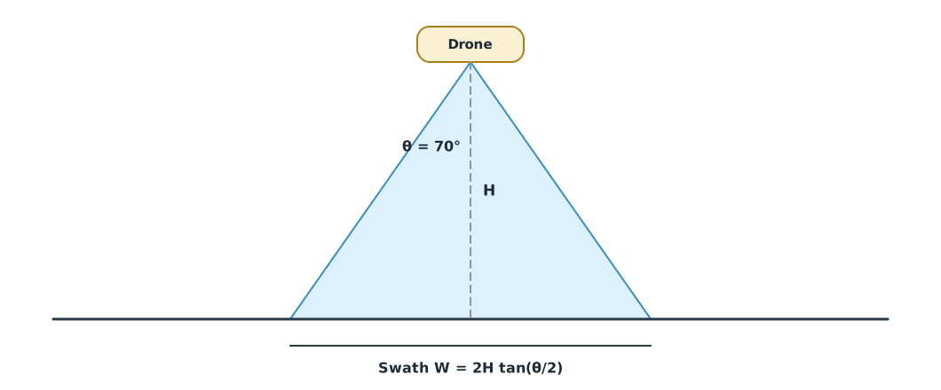
Example 1 Pulse density of three LiDAR setups
Assume a single pass with no overlap, pulses spread evenly, and one pulse counted per shot.
import math

def pulse_density(prr, h, v, fov_deg):
    swath = 2 * h * math.tan(math.radians(fov_deg / 2))
    return swath, prr / (v * swath)

cases = [
    ("solid-state 240k", 240_000, 60, 8, 70),
    ("same, higher and faster", 240_000, 120, 15, 70),
    ("small mechanical 20k", 20_000, 100, 12, 70),
]
for name, prr, h, v, fov in cases:
    w, d = pulse_density(prr, h, v, fov)
    level = "meets QL1" if d >= 8 else "meets QL2" if d >= 2 else "below QL2"
    print(f"{name:<24} swath {w:5.1f} m, {d:6.1f} pulses/m^2, spacing {1 / math.sqrt(d):.2f} m, {level}")
solid-state 240k swath 84.0 m, 357.0 pulses/m^2, spacing 0.05 m, meets QL1
same, higher and faster swath 168.0 m, 95.2 pulses/m^2, spacing 0.10 m, meets QL1
small mechanical 20k swath 140.0 m, 11.9 pulses/m^2, spacing 0.29 m, meets QL1Flying higher and faster covers more area per flight, but density falls by the product of both. A low-rate sensor can still meet QL1 if it flies slowly enough. In practice, overlapping passes raise density, while the edges of the scan and non-reflective surfaces lower it.
LiDAR uses lasers, so check the laser safety class under IEC 60825-1:2014 in the manufacturer’s documentation before operating near people, especially during ground tests.
FMCW radar
A millimetre-wave FMCW (frequency-modulated continuous wave) radar transmits a wave whose frequency rises linearly, called a chirp. The reflection returns delayed by ; mixing it with the wave currently being transmitted gives a beat frequency , where is the chirp slope. Texas Instruments’ SPYY005A shows that range resolution depends only on chirp bandwidth, . Radar works in dust, smoke, fog and darkness, so it is popular as an altimeter and obstacle sensor on agricultural drones.
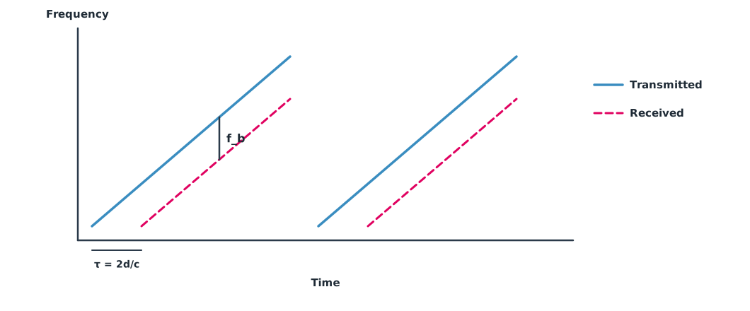
Example 2 Range resolution and beat frequency
C = 299_792_458

for bw in (4e9, 1e9, 250e6):
    print(f"bandwidth {bw / 1e9:.2f} GHz -> range resolution {C / (2 * bw) * 100:.2f} cm")
S = 30e12                                   # Hz/s chirp slope (30 MHz/µs)
for d in (5, 10, 20):
    print(f"target at {d:>2} m -> beat frequency {S * 2 * d / C / 1e6:.2f} MHz")
bandwidth 4.00 GHz -> range resolution 3.75 cm
bandwidth 1.00 GHz -> range resolution 14.99 cm
bandwidth 0.25 GHz -> range resolution 59.96 cm
target at 5 m -> beat frequency 1.00 MHz
target at 10 m -> beat frequency 2.00 MHz
target at 20 m -> beat frequency 4.00 MHzA 4 GHz bandwidth gives 3.75 cm resolution, matching the example in TI’s document, and range is proportional to beat frequency, so the radar separates ranges by separating frequencies.
Choosing a sensor for the mission
The hypothetical mission is measuring sugarcane canopy height over a 50-rai plot with the lab’s VTOL drone. A weighted scoring matrix helps the team decide transparently, but the result depends on the weights, so always try changing them.
Example 3 Scoring matrix and sensitivity to weights
Scores from 1 to 5 agreed by the team (hypothetical values).
criteria = ["height accuracy", "sees ground under crop", "mass on VTOL", "cost", "processing effort"]
scores = {
    "LiDAR": [5, 5, 2, 1, 3],
    "RGB photogrammetry": [3, 1, 5, 5, 3],
    "mmWave radar altimeter": [2, 2, 4, 4, 4],
}
weight_sets = {
    "accuracy first": [0.35, 0.25, 0.15, 0.15, 0.10],
    "budget first": [0.15, 0.25, 0.15, 0.35, 0.10],
}
for label, w in weight_sets.items():
    assert abs(sum(w) - 1) < 1e-9
    ranked = sorted(((sum(a * b for a, b in zip(w, s)), name) for name, s in scores.items()), reverse=True)
    print(f"{label}: " + ", ".join(f"{name} {total:.2f}" for total, name in ranked))
accuracy first: LiDAR 3.75, RGB photogrammetry 3.10, mmWave radar altimeter 2.80
budget first: RGB photogrammetry 3.50, mmWave radar altimeter 3.20, LiDAR 2.95When accuracy matters most, LiDAR wins; when budget carries the most weight, RGB photography comes first. The team must agree the weights from the data users’ needs before looking at scores, and record the reasons.
Using several sensors together requires time synchronisation. For a LiDAR firing hundreds of thousands of points per second on a drone flying at 10 m/s, a 10 ms timing error shifts points by 10 cm. Real systems use the GNSS PPS signal or a time-synchronisation protocol (Groves, 2013).
Module lab
Lab: planning mission sensors
- Use the code from Example 1 with the specification of a LiDAR the lab has or plans to buy, and find the altitude and speed that meet QL1.
- If the lab has sample LiDAR data, open it in CloudCompare, count the real density and compare with the calculation.
- Test a radar development board indoors and record the ranges it can separate, compared with Example 2.
- Build a scoring matrix for your group’s own mission, have each member set weights independently and compare results.
- Check the laser safety class in the manufacturer’s documentation before testing near people.
Common mistakes
Watch out
- Choosing a sensor before framing the mission question.
- Using the advertised pulse rate without accounting for altitude, speed and field of view.
- Treating radar range resolution as accuracy.
- Setting the matrix weights after seeing the results.
- Not synchronising time between sensors.
Summary
- LiDAR ranges with pulse timing; pulse density = PRR/(v·W), compared with quality levels such as QL1 ≥ 8 pulses/m².
- FMCW radar separates ranges by beat frequency, with range resolution c/2B.
- A weighted scoring matrix helps choose sensors, but its sensitivity to the weights must be checked.
- Multiple sensors need time synchronisation, and LiDAR needs its laser safety class checked.
Check your understanding
- Flying at 50 m with a 90° field of view, how wide is the swath?
- PRR 100,000 pulses/s, speed 10 m/s, swath 100 m: what is the density, and does it meet QL1?
- What range resolution does a 2 GHz chirp bandwidth give?
- If both altitude and speed double, by what factor does pulse density change?
- A drone flies at 12 m/s and the LiDAR–IMU timing is off by 5 ms. How large is the position error?
Answers
- m
- pulses/m², which meets QL1.
- m, or 7.5 cm
- It falls to a quarter, because the swath and the speed both double.
- m
Key formulas
| Swath width and pulse density | |
| FMCW range resolution | |
| Beat frequency |
Key references
- U.S. Geological Survey. (2025). Lidar base specification tables (2025 rev. A). link
- Iovescu, C., & Rao, S. (2020). The fundamentals of millimeter wave radar sensors (SPYY005A). Texas Instruments. link
- International Electrotechnical Commission. (2014). Safety of laser products – Part 1: Equipment classification and requirements (IEC 60825-1:2014, Ed. 3.0). link
- Fraden, J. (2016). Handbook of modern sensors: Physics, designs, and applications (5th ed.). Springer. link
- Groves, P. D. (2013). Principles of GNSS, inertial, and multisensor integrated navigation systems (2nd ed.). Artech House. link
Further reading
Study the assigned knowledge units in advance, review media and take the module quiz
LiDAR, radar and obstacle-avoidance sensors
Payloads and survey data quality
In class / field
Lab or field practice from worksheets with a safety checklist
Learning evidence: Checked worksheets and quiz results