State estimation and EKF
UAT 305 Autopilot and Control Technology
Lesson
By the end of this module you will be able to
- Explain the predict and update steps of a Kalman filter
- Write a Kalman filter that estimates height from an accelerometer and a barometer
- Compute innovation test ratios and decide whether data is used or rejected
- Read EKF3 consistency values in ArduPilot logs
Why this matters
An autopilot does not know its position and attitude directly; it estimates them from several sensors that each have weaknesses. An accelerometer responds quickly but drifts when integrated for long because of bias. A barometer does not drift but is noisy. GNSS is accurate over time but updates slowly and can drop out. A Kalman filter combines the strengths of all of them. The drone knowledge base’s unit on state estimation with the Kalman filter and EKF covers fusing IMU, GNSS and barometer and diagnosing the EKF, and Groves’s textbook explains multisensor integrated navigation in depth.
The two steps of a Kalman filter
Following Welch and Bishop’s introduction, a Kalman filter repeats two steps. The predict step uses the model and input (such as measured acceleration) to predict the next state, with an uncertainty that grows with the process noise . The update step compares the measurement with the prediction; the difference is the innovation, and the state is adjusted by the Kalman gain , which weighs the prediction uncertainty against the measurement uncertainty . The EKF (extended Kalman filter) uses the same idea with a nonlinear model, linearised around the current state.
Example 1 Height from an accelerometer and a barometer
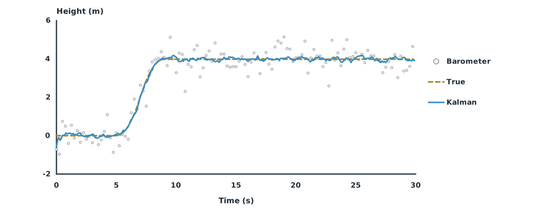
A drone hovers and then climbs 4 m between seconds 5 and 9. The accelerometer has a 0.05 m/s² bias and 0.3 m/s² noise; the barometer has 0.5 m noise (simulated data).
import numpy as np

rng = np.random.default_rng(3)
dt, T = 0.01, 30.0
n = int(T / dt)
t = np.arange(n) * dt
true_a = np.where((t > 5) & (t < 7), 1.0, 0.0) - np.where((t > 7) & (t < 9), 1.0, 0.0)
true_v = np.cumsum(true_a) * dt
true_h = np.cumsum(true_v) * dt
acc = true_a + 0.05 + rng.normal(0, 0.3, n)    # m/s² with bias
baro = true_h + rng.normal(0, 0.5, n)          # m

A = np.array([[1, dt], [0, 1]])                # state [height, velocity]
B = np.array([0.5 * dt * dt, dt])
H = np.array([[1.0, 0.0]])
Q = np.diag([1e-5, 1e-3])
R = np.array([[0.25]])
x, P, est = np.zeros(2), np.eye(2), []
for k in range(n):
    x = A @ x + B * acc[k]                     # predict
    P = A @ P @ A.T + Q
    S = H @ P @ H.T + R                        # update
    K = P @ H.T @ np.linalg.inv(S)
    x = x + (K @ (baro[k] - H @ x)).ravel()
    P = (np.eye(2) - K @ H) @ P
    est.append(x[0])

rms = lambda e: float(np.sqrt(np.mean(e ** 2)))
drift = (np.cumsum(np.cumsum(acc) * dt) * dt)[-1] - true_h[-1]
print(f"true height at end {true_h[-1]:.2f} m")
print(f"accelerometer only: error at end {drift:.1f} m")
print(f"barometer only: RMS error {rms(baro - true_h):.2f} m")
print(f"Kalman filter: RMS error {rms(np.array(est) - true_h):.2f} m")
true height at end 3.98 m
accelerometer only: error at end 26.7 m
barometer only: RMS error 0.50 m
Kalman filter: RMS error 0.08 mThe accelerometer alone drifts by tens of metres in 30 seconds because a small bias is integrated twice. The barometer alone jitters by about half a metre. The Kalman filter’s error is several times smaller than either, because it uses acceleration for short-term changes and the barometer to pull the estimate back over the long term.
Testing innovations before using data
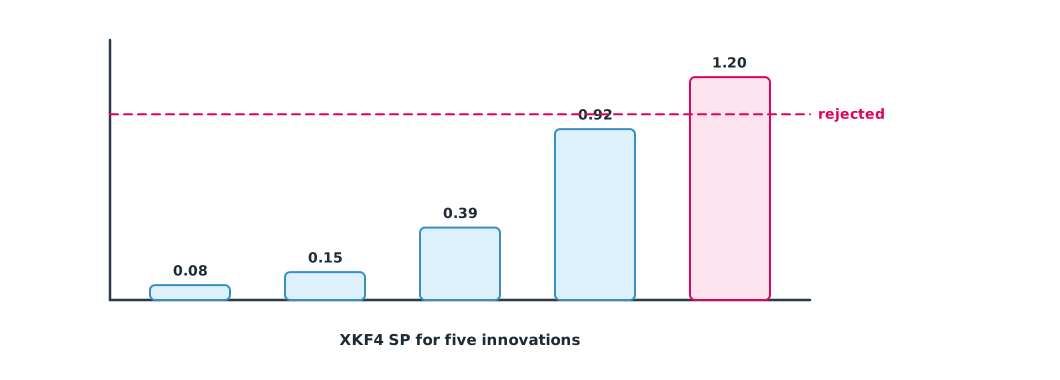
ArduPilot’s EKF3 does not use every measurement. Before updating, it checks whether the innovation is larger than the uncertainty allows. In the 4.6.3 source code, the test ratio is the innovation squared divided by the innovation variance times (gate/100)², and it must be below 1 for the data to be used. The gates are set with EK3_POS_I_GATE, EK3_VEL_I_GATE and EK3_HGT_I_GATE (default 500, i.e. 5 standard deviations) and EK3_MAG_I_GATE (default 300). The XKF4 log message records the square root of this ratio in the SV, SP, SH and SM fields, so a value above 1 means the data was rejected, while XKF3 records the innovations themselves.
Example 2 Which GNSS positions are rejected?
The position innovation variance is 4 m² (2 m standard deviation) and the gate is 500 (simulated data).
import math

GATE, S = 500, 4.0                             # EK3_POS_I_GATE, m²
innovations = [0.8, -1.5, 3.9, 9.2, 12.0]      # m
for nu in innovations:
    ratio = nu ** 2 / (S * (GATE / 100) ** 2)
    logged = math.sqrt(ratio)                  # value seen in XKF4.SP
    print(f"innovation {nu:+5.1f} m: test ratio {ratio:.3f}, logged {logged:.2f} -> {'used' if ratio < 1 else 'REJECTED'}")
print(f"largest accepted innovation: {GATE / 100 * math.sqrt(S):.1f} m")
innovation +0.8 m: test ratio 0.006, logged 0.08 -> used
innovation -1.5 m: test ratio 0.022, logged 0.15 -> used
innovation +3.9 m: test ratio 0.152, logged 0.39 -> used
innovation +9.2 m: test ratio 0.846, logged 0.92 -> used
innovation +12.0 m: test ratio 1.440, logged 1.20 -> REJECTED
largest accepted innovation: 10.0 mValues more than 5 standard deviations from the prediction are rejected, which protects the EKF from GNSS jumps caused by multipath. But if data is rejected for a long time, the EKF drifts on the accelerometer and may reset to the new GNSS value. Widening the gate to “stop the warnings” is therefore not a fix; find out why the values disagree.
Module lab
Lab: reading EKF health
- Change and in Example 1 and observe when the filter trusts the barometer or the accelerometer more
- Open a SITL log and look at the SV, SP, SH and SM fields of XKF4 over the flight
- Simulate a GPS glitch in SITL and see when SP exceeds 1 and what the EKF does
- Compute the largest accepted innovation with Example 2 from the variances in the log
- Write a summary of how to read EKF health for the field team
Common mistakes
Watch out
- Believing one sensor’s reading is the truth
- Widening the gate to silence warnings
- Reading the XKF4 values as variances when they are square-root test ratios
- Setting a sensor’s smaller than reality, so the filter chases noise
- Overlooking vibration, which corrupts acceleration and damages the EKF
Summary
- A Kalman filter predicts with a model and input, then updates with measurements, weighting by uncertainty
- Fusing an accelerometer with a barometer gives a more accurate height than either alone
- EKF3 uses data when the test ratio is below 1; a gate of 500 means 5 standard deviations
- The XKF4 SV, SP, SH and SM fields are square-root test ratios; values above 1 mean rejection
Check your understanding
- Why does integrating acceleration alone drift?
- If the barometer’s increases, does the filter trust the barometer more or less?
- Innovation 6 m, variance 4 m², gate 500. What is the test ratio?
- What does an SP value of 0.6 in the log mean?
- Why should EKF warnings not be fixed by widening the gate?
Answers
- A small bias is integrated twice, so the error grows with the square of time
- Less
- The innovation is at 60% of the gate boundary, and the data is used
- Wrong data would be used and corrupt the estimate; the cause of the disagreement must be found
Key formulas
| Predict step | |
| Update step | |
| EKF3 test ratio |
Key references
- Welch, G., & Bishop, G. (2004). An introduction to the Kalman filter (TR 95-041). University of North Carolina at Chapel Hill. link
- Groves, P. D. (2013). Principles of GNSS, inertial, and multisensor integrated navigation systems (2nd ed.). Artech House. link
- ArduPilot Dev Team. Extended Kalman filter (EKF) overview. ArduPilot Copter documentation. link
- ArduPilot Dev Team. Onboard message log messages. ArduPilot Copter documentation. link
- ArduPilot Dev Team. ArduPilot source code, tag Copter-4.6.3 [Computer software]. GitHub. link
- PX4 Autopilot. Using the ECL EKF. PX4 user guide (main). link
Further reading
Study the assigned knowledge units in advance, review media and take the module quiz
State estimation with Kalman filters/EKF
GNSS and constrained navigation
In class / field
Lab or field practice from worksheets with a safety checklist
Learning evidence: Checked worksheets and quiz results