Path planning and avoidance

Example 1 Crossing panel rows to the inverter cabinet

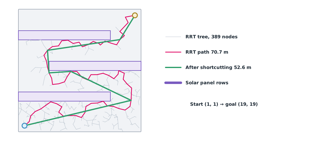
A 20 × 20 m area has three panel rows staggered from alternate sides. The UGV starts at (1, 1) and must reach the inverter cabinet at (19, 19). The branch step is 1 m, 10% of samples are the goal, and the random seed is fixed so results repeat (simulated data).

import numpy as np

rng = np.random.default_rng(7)
start, goal = np.array([1.0, 1.0]), np.array([19.0, 19.0])
# solar panel rows (xmin, ymin, xmax, ymax) m
rows = [(0, 5, 15, 6.5), (5, 10, 20, 11.5), (0, 15, 15, 16.5)]

def free(p):
    return all(not (x0 <= p[0] <= x1 and y0 <= p[1] <= y1) for x0, y0, x1, y1 in rows)

def segment_free(a, b, step=0.1):
    n = max(2, int(np.linalg.norm(b - a) / step))
    return all(free(a + (b - a) * s) for s in np.linspace(0, 1, n))

def rrt(max_nodes=3000, step=1.0, goal_bias=0.1):
    nodes, parent = [start], [-1]
    while len(nodes) < max_nodes:
        sample = goal if rng.random() < goal_bias else rng.uniform(0, 20, 2)
        i = int(np.argmin([np.linalg.norm(n - sample) for n in nodes]))
        d = sample - nodes[i]
        new = nodes[i] + d / max(np.linalg.norm(d), 1e-9) * min(step, np.linalg.norm(d))
        if free(new) and segment_free(nodes[i], new):
            nodes.append(new); parent.append(i)
            if np.linalg.norm(new - goal) < step and segment_free(new, goal):
                nodes.append(goal); parent.append(len(nodes) - 2)
                path, k = [], len(nodes) - 1
                while k != -1:
                    path.append(nodes[k]); k = parent[k]
                return path[::-1], len(nodes)
    return None, len(nodes)

def length(path):
    return sum(np.linalg.norm(path[i+1] - path[i]) for i in range(len(path) - 1))

def shortcut(path):
    out, i = [path[0]], 0
    while i < len(path) - 1:
        j = len(path) - 1
        while j > i + 1 and not segment_free(path[i], path[j]):
            j -= 1
        out.append(path[j]); i = j
    return out

path, n = rrt()
short = shortcut(path)
print(f"nodes in tree {n}")
print(f"RRT path {length(path):.1f} m ({len(path)} points)")
print(f"after shortcutting {length(short):.1f} m ({len(short)} points)")
print(f"straight line {np.linalg.norm(goal - start):.1f} m (blocked by panels)")

nodes in tree 389
RRT path 70.7 m (74 points)
after shortcutting 52.6 m (7 points)
straight line 25.5 m (blocked by panels)

RRT finds a feasible path within a few hundred nodes, but it winds for 70.7 m. Shortcutting cuts it to 52.6 m with just 7 waypoints. The path still hugs the panel edges, so real work must inflate obstacles by half the vehicle width plus a margin before planning. RRT results depend on sampling: a different seed gives a different path, so test several times.

Example 2 Joining a panel row line with a 0.3 s steering delay

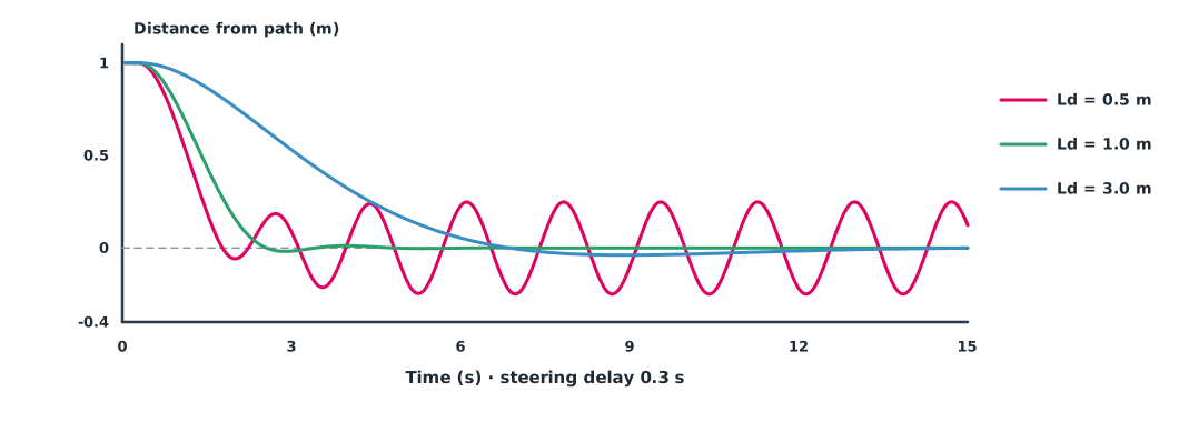
The UGV drives at 1 m/s, starting 1.0 m from the row line and parallel to it. Steering commands reach the wheels 0.3 s late because of communication and the motor driver. Compare lookahead distances of 0.5, 1.0, 1.5 and 3.0 m (a kinematic model).

import numpy as np

V, DT, T = 1.0, 0.05, 15.0     # speed m/s, time step s, simulated time s
DELAY = 0.3                    # steering command reaches wheels 0.3 s late

def track(Ld):
    x, y, th = 0.0, 1.0, 0.0            # start 1.0 m from the path y = 0
    buf = [0.0] * int(round(DELAY / DT))
    ys = []
    for _ in range(int(T / DT)):
        dx, dy = Ld, -y                 # goal point on the path, Ld ahead along x
        alpha = np.arctan2(dy, dx) - th
        buf.append(2 * np.sin(alpha) / np.hypot(dx, dy))
        kappa = buf.pop(0)
        th += V * kappa * DT
        x += V * np.cos(th) * DT
        y += V * np.sin(th) * DT
        ys.append(y)
    return np.array(ys)

for Ld in [0.5, 1.0, 1.5, 3.0]:
    ys = track(Ld)
    out = np.where(np.abs(ys) >= 0.05)[0]
    settle = (out[-1] + 1) * DT
    s = f"settles within ±5 cm by {settle:.1f} s" if settle < T else "does not settle in 15 s"
    print(f"Ld={Ld:.1f} m  {s}  max overshoot {max(0, -ys.min())*100:.1f} cm")

Ld=0.5 m  does not settle in 15 s  max overshoot 24.9 cm
Ld=1.0 m  settles within ±5 cm by 2.3 s  max overshoot 1.8 cm
Ld=1.5 m  settles within ±5 cm by 3.2 s  max overshoot 2.7 cm
Ld=3.0 m  settles within ±5 cm by 6.1 s  max overshoot 3.8 cm

Without delay, the shortest lookahead joins the path fastest. With a 0.3 s delay, a 0.5 m lookahead oscillates without settling, 1.0 m reaches the ±5 cm band fastest, and 3.0 m is smooth but slow. Lookahead must therefore be chosen together with the speed and delay of the real system; many systems scale lookahead with speed.