Thermal and LiDAR
UAT 362 Unmanned Aircraft Systems Technology for Industrial, Energy and Infrastructure Applications
Lesson
By the end of this module you will be able to
- Choose distance and thermal camera so the pixel size is small enough for the inspection target
- Explain LiDAR ranging and compute pulse density against USGS quality levels
- Compute distances from a point cloud to a conductor for vegetation management
- Explain the use of UV cameras for corona and the limits of each sensor
Why this matters
UAT 361 covered the basics of thermal imaging. This course extends it to energy systems, which need several sensors together. Thermal cameras find hot joints, LiDAR measures tree-to-conductor distances more precisely than photographs, and UV cameras see corona that eyes and ordinary cameras cannot. Each sensor has limits, and a wrong choice misses defects or raises false alarms.
Thermal cameras in energy work
Thermal cameras have far fewer pixels than colour cameras. A small hot spot such as a line joint must cover several pixels for a reliable temperature, because a pixel that covers both the joint and the sky averages to a value below the true one. The team must set the required pixel size and compute the distance as in UAT 361 module 4. NETD gives the sensitivity to temperature differences, while emissivity and reflected temperature must suit the material. Shiny conductor metal has low emissivity and can reflect the cold sky strongly, so it is easy to misread (Vollmer and Möllmann).
LiDAR
LiDAR fires laser pulses and measures their round-trip time. The range is because the light travels both ways. A drone system sweeps the beam across a swath as it flies, so the pulse density on the ground is roughly the pulse repetition frequency (PRF) divided by the area swept per second.
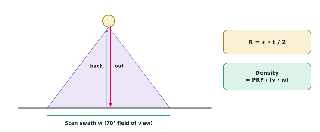
The USGS Lidar Base Specification defines quality levels for LiDAR data, for example QL2 with at least 2 pulses/m² and QL1 with at least 8 pulses/m². These were written for wide-area surveys but are a useful reference when stating data quality.
Example 1. Travel time and pulse density
Assumed LiDAR: PRF 240,000 pulses/s, 70° field of view.
import math

C = 299_792_458                     # m/s
PRF, FOV_DEG = 240_000, 70

for height, speed in ((60, 6.0), (100, 12.0)):
    t_ns = 2 * height / C * 1e9
    swath = 2 * height * math.tan(math.radians(FOV_DEG / 2))
    density = PRF / (speed * swath)
    level = "QL1" if density >= 8 else ("QL2" if density >= 2 else "below QL2")
    print(f"H {height} m, v {speed} m/s: echo {t_ns:.0f} ns, swath {swath:.1f} m, "
          f"{density:.0f} pulses/m2 ({level})")
H 60 m, v 6.0 m/s: echo 400 ns, swath 84.0 m, 476 pulses/m2 (QL1)
H 100 m, v 12.0 m/s: echo 667 ns, swath 140.0 m, 143 pulses/m2 (QL1)A low-flying drone LiDAR therefore far exceeds the density thresholds, but density is not everything. Position accuracy still depends on GNSS/INS and calibration, and a thin conductor may return only a few points.
Tree clearance from conductors
Trees growing close to a line cause faults and outages. The North American standard NERC FAC-003-5 sets a minimum vegetation clearance distance (MVCD) by voltage and altitude, an example of a clearly defined criterion. In Thailand the criteria of the utility operating the line apply. A LiDAR point cloud makes it possible to compute the distance from every tree top to the conductor.
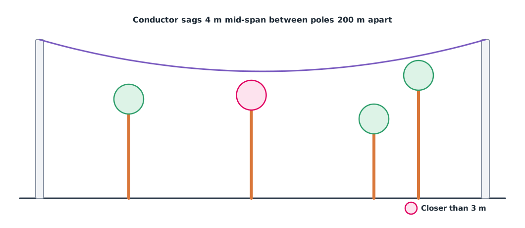
Example 2. Distance from tree tops to a sagging conductor
The conductor sags 4 m mid-way along a 200 m span, modelled as a parabola. The 3 m criterion is assumed for this lesson.
import math

def wire_z(x):                      # conductor height (m) at distance x from the first pole
    return 20 - 4 * (1 - ((x - 100) / 100) ** 2)

wire = [(x / 10, 0.0, wire_z(x / 10)) for x in range(0, 2001)]
trees = {"T1": (40, 3, 14.5), "T2": (95, -2, 15.0), "T3": (150, 4, 12.0), "T4": (170, -6, 17.5)}
LIMIT = 3.0
for name, top in trees.items():
    d = min(math.dist(top, p) for p in wire)
    print(f"{name}: {d:.2f} m {'-> trim' if d < LIMIT else ''}")
T1: 4.20 m
T2: 2.24 m -> trim
T3: 6.40 m
T4: 6.02 mT4 is the tallest but stands 6 m to the side, so it is not the closest. T2 is shorter but sits under the middle of the span where the conductor hangs lowest. In a side view these two look the opposite of reality, so a 3D calculation is essential. In practice, extra sag when the conductor is hot and swing in the wind must also be considered.
UV cameras for corona
Corona discharge is partial discharge around damaged or dirty high-voltage conductors or insulators, and it emits ultraviolet light. Studies by Wang and Qian (2019) and Wang and colleagues (2014) used solar-blind UV cameras working below about 280 nm, where sunlight is filtered out by the atmosphere, so corona can be seen even in daylight. A UV camera shows where discharge occurs, but judging its severity needs specialists and other data.
Module lab
Lab: point clouds and conductor clearance
- Open a sample point cloud (or the one from UAT 361 module 3) in CloudCompare or QGIS and check the real density in several areas
- Use Example 1 with the specifications of an available LiDAR to compute density at different heights and speeds
- In data with a conductor or reference line, separate conductor and tree points and compute distances with Example 2
- Explain why a side view alone misjudges distances
- List trees to be trimmed according to the line owner’s criterion (or the instructor’s assumed criterion)
Common mistakes
Watch out
- Reading hot spots smaller than a pixel, giving temperatures that are too low
- Reading shiny metal without considering emissivity and reflection
- Confusing pulses per square metre with position accuracy
- Judging tree clearance from a side view without lateral distance
- Using foreign clearance criteria instead of the Thai utility’s
Summary
- Hot spots must cover several pixels, and emissivity must suit the material
- LiDAR measures R = c·t/2; density is about PRF/(v·w) and can be compared with USGS quality levels
- Tree-to-conductor distance must be computed in 3D against the line owner’s criterion
- Solar-blind UV cameras see corona in daylight
Check your understanding
- A LiDAR measures a round-trip time of 500 ns. What is the range?
- At 80 m with a 70° field of view, how wide is the swath?
- PRF 100,000 pulses/s at 10 m/s with a 100 m swath. What is the density, and which level does it meet?
- Why is the tallest tree not necessarily closest to the conductor?
- Why can solar-blind UV cameras be used in daylight?
Answers
- m
- m
- pulses/m², meeting QL1
- Distance also depends on lateral position and the conductor sag at that point
- They work in a band where sunlight is filtered out by the atmosphere
Key formulas
| Range from time of flight | |
| Scan swath | |
| Pulse density (approximate) |
Key references
- Vollmer, M., & Möllmann, K.-P. (2017). Infrared thermal imaging: Fundamentals, research and applications (2nd ed.). Wiley-VCH. link
- Teledyne FLIR. Comparing sensitivity of thermal imaging cameras and modules (NETD). link
- U.S. Geological Survey. (2025). Lidar base specification tables (2025 rev. A). link
- North American Electric Reliability Corporation. (2021). Transmission vegetation management (Reliability Standard FAC-003-5). link
- Wang, Y., & Qian, Y. (2019). Characteristics of the corona discharge of polymer insulators based on solar-blind ultraviolet images. Optical Engineering, 58(11), 113102. link
- Wang, S., Lv, F., & Liu, Y. (2014). Estimation of discharge magnitude of composite insulator surface corona discharge based on ultraviolet imaging method. IEEE Transactions on Dielectrics and Electrical Insulation, 21(4), 1697–1704. link
- Siegwart, R., Nourbakhsh, I. R., & Scaramuzza, D. (2011). Introduction to autonomous mobile robots (2nd ed.). MIT Press. link
- Fraden, J. (2016). Handbook of modern sensors: Physics, designs, and applications (5th ed.). Springer. link
Further reading
Study the assigned knowledge units in advance, review media and take the module quiz
Principles of thermal imaging
LiDAR, radar and obstacle-avoidance sensors
In class / field
Intensive lab and field practice recorded in a lab notebook
Learning evidence: Lab notebook signed by the instructor