SLAM and sensor fusion
UAT 366 Indoor Autonomous and Multi-Unmanned Aircraft Systems
Lesson
By the end of this module you will be able to
- Explain the predict and update steps of a two-state Kalman filter (position and velocity)
- Fuse the IMU with UWB position and read how the variance shrinks when a measurement arrives
- Explain graph-based SLAM and loop closure
- Distribute the loop-closure error to correct the whole path
Why this matters
The IMU gives very frequent data but drifts quickly. UWB gives position that does not drift, but it is noisy and slower. The Kalman filter (Kalman, 1960) fuses the strengths of both. UAT 322 covered a one-state Kalman filter; this module uses two states, position and velocity, to show how position measurements let us estimate a velocity that is never measured directly. When there is no UWB at all, SLAM and loop closure help correct accumulated drift.
A two-state Kalman filter
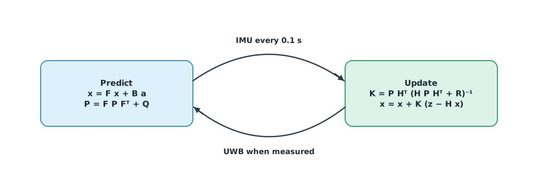
The state is , position and velocity along the aisle. The predict step uses IMU acceleration every 0.1 s, and the uncertainty grows each time. The update step uses the UWB position when a measurement arrives, and the uncertainty shrinks. The textbooks by Thrun et al. (2005) and Groves (2013) give the full equations.
Example 1 Fusing the IMU with UWB
The drone flies along an aisle at a true speed of 1.0 m/s, starting with a velocity estimate of 0 (unknown). UWB measures position every 0.5 s with a standard deviation of 0.10 m. The measurement errors use a fixed list so the results are repeatable.
DT, SIGMA_A, SIGMA_Z = 0.1, 0.5, 0.10
uwb_noise = [0.08, -0.12, 0.05, 0.10, -0.06, -0.09]      # m, fixed values standing in for noise

x = [0.0, 0.0]                                            # position, velocity (estimate)
P = [[0.5 ** 2, 0.0], [0.0, 1.0 ** 2]]
q = SIGMA_A ** 2
Q = [[q * DT ** 4 / 4, q * DT ** 3 / 2], [q * DT ** 3 / 2, q * DT ** 2]]

for step in range(1, 31):
    x = [x[0] + DT * x[1], x[1]]                           # predict (IMU measures zero acceleration)
    P = [[P[0][0] + DT * (P[1][0] + P[0][1]) + DT * DT * P[1][1] + Q[0][0], P[0][1] + DT * P[1][1] + Q[0][1]],
         [P[1][0] + DT * P[1][1] + Q[1][0], P[1][1] + Q[1][1]]]
    if step % 5 == 0:                                      # update with UWB
        z = 1.0 * step * DT + uwb_noise[step // 5 - 1]
        s = P[0][0] + SIGMA_Z ** 2
        k = [P[0][0] / s, P[1][0] / s]
        innov = z - x[0]
        x = [x[0] + k[0] * innov, x[1] + k[1] * innov]
        P = [[(1 - k[0]) * P[0][0], (1 - k[0]) * P[0][1]], [P[1][0] - k[1] * P[0][0], P[1][1] - k[1] * P[0][1]]]
        print(f"t {step * DT:.1f} s: p {x[0]:.2f} (true {step * DT:.2f}), v {x[1]:.2f}, "
              f"sigma_p {P[0][0] ** 0.5:.3f} m, sigma_v {P[1][1] ** 0.5:.3f} m/s")
t 0.5 s: p 0.57 (true 0.50), v 0.57, sigma_p 0.099 m, sigma_v 0.719 m/s
t 1.0 s: p 0.88 (true 1.00), v 0.61, sigma_p 0.097 m, sigma_v 0.262 m/s
t 1.5 s: p 1.48 (true 1.50), v 0.98, sigma_p 0.090 m, sigma_v 0.164 m/s
t 2.0 s: p 2.06 (true 2.00), v 1.07, sigma_p 0.085 m, sigma_v 0.141 m/s
t 2.5 s: p 2.49 (true 2.50), v 0.97, sigma_p 0.082 m, sigma_v 0.137 m/s
t 3.0 s: p 2.93 (true 3.00), v 0.92, sigma_p 0.081 m, sigma_v 0.136 m/sThe velocity, never measured directly, is estimated from successive position measurements and approaches 1.0 m/s within a few seconds. The position standard deviation falls below the UWB error itself, because the filter combines many measurements.
Graph-based SLAM and loop closure
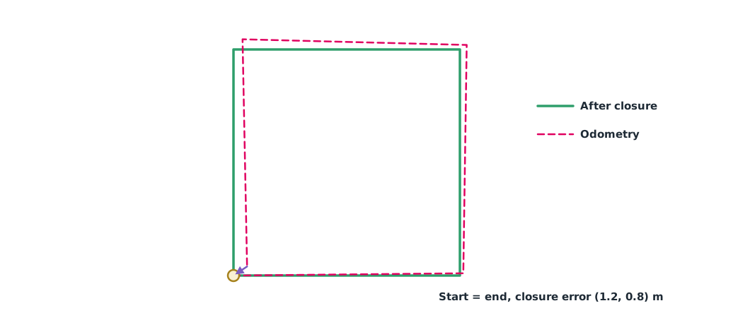
SLAM (simultaneous localization and mapping) builds a map and localises within it at the same time. The tutorial by Grisetti et al. (2010) describes graph-based SLAM, which stores each pose as a node and odometry relations as edges. When the drone sees a place again (loop closure), it gains a new edge saying the end point and start point are the same place, and the accumulated error around the loop is spread across every node. Systems such as ORB-SLAM3 do this with large numbers of images.
Example 2 Distributing the loop-closure error by distance
This simple method spreads the error in proportion to cumulative distance. Real systems optimise the whole graph, weighting each edge by its uncertainty.
import math

odom = [(0.0, 0.0), (20.3, 0.2), (20.6, 20.4), (0.8, 20.9), (1.2, 0.8)]   # truly returns to the start
err = (odom[-1][0] - odom[0][0], odom[-1][1] - odom[0][1])
seg = [math.dist(a, b) for a, b in zip(odom, odom[1:])]
cum = [0.0]
for s in seg:
    cum.append(cum[-1] + s)
total = cum[-1]
print(f"loop closure error ({err[0]:.1f}, {err[1]:.1f}) m over {total:.1f} m = {math.hypot(*err) / total:.1%}")
for (x, y), s in zip(odom, cum):
    f = s / total
    print(f"({x:5.1f}, {y:5.1f}) -> ({x - f * err[0]:5.2f}, {y - f * err[1]:5.2f})")
loop closure error (1.2, 0.8) m over 80.4 m = 1.8%
( 0.0, 0.0) -> ( 0.00, 0.00)
( 20.3, 0.2) -> (20.00, -0.00)
( 20.6, 20.4) -> (20.00, 20.00)
( 0.8, 20.9) -> (-0.10, 20.30)
( 1.2, 0.8) -> ( 0.00, 0.00)Module lab
Lab: fusion and loop closure
- Log the IMU and UWB position while flying along an aisle in the lab.
- Apply the code from Example 1 to the real data, adjust SIGMA_A and SIGMA_Z, and observe the effect on velocity and variance.
- Compare with the EKF2 output in the PX4 log and explain the differences.
- Fly a loop back to the start on VIO, measure the loop-closure error and use the code from Example 2 to correct the path.
- Compare the result with the SLAM system available in the lab (such as ORB-SLAM3) using the trajectory evaluation method from UAT 322.
Common mistakes
Watch out
- Setting the measurement variance lower than reality, so the filter trusts UWB too much.
- Forgetting Q, so the variance shrinks to zero and new measurements are ignored.
- Using sensor timestamps from different clocks without synchronising them.
- Trusting a false loop closure, which warps the entire map.
- Judging by how the plot looks instead of by error numbers.
Summary
- A two-state Kalman filter predicts with the IMU and updates with UWB; variance grows on prediction and shrinks on update.
- Position measurements let the filter estimate velocity that is never measured directly.
- Graph-based SLAM stores poses as nodes and relations as edges.
- Loop closure adds information that spreads the accumulated error along the whole path.
Check your understanding
- In the predict step, does the variance P grow or shrink, and why?
- If P[0][0] = 0.04 m² and the measurement variance is 0.01 m², what is the position gain K?
- A loop-closure error of (3, 4) m on a 100 m loop is what percentage?
- From question 3, how far must the node at a cumulative distance of 50 m move?
- What does a loop closure matched to the wrong place cause?
Answers
- It grows, because prediction accumulates uncertainty from Q and from the uncertain velocity.
- Half the error, (1.5, 2) m.
- The map and path warp, because the graph is forced to join two places that are not the same.
Key formulas
| Predict step | |
| Update step | |
| Distributing the loop-closure error |
Key references
- Kalman, R. E. (1960). A new approach to linear filtering and prediction problems. Journal of Basic Engineering, 82(1), 35–45. link
- Thrun, S., Burgard, W., & Fox, D. (2005). Probabilistic robotics. MIT Press. link
- Groves, P. D. (2013). Principles of GNSS, inertial, and multisensor integrated navigation systems (2nd ed.). Artech House. link
- Grisetti, G., Kümmerle, R., Stachniss, C., & Burgard, W. (2010). A tutorial on graph-based SLAM. IEEE Intelligent Transportation Systems Magazine, 2(4), 31–43. link
- Cadena, C., Carlone, L., Carrillo, H., Latif, Y., Scaramuzza, D., Neira, J., Reid, I., & Leonard, J. J. (2016). Past, present, and future of simultaneous localization and mapping: Toward the robust-perception age. IEEE Transactions on Robotics, 32(6), 1309–1332. link
- Campos, C., Elvira, R., Gómez Rodríguez, J. J., Montiel, J. M. M., & Tardós, J. D. (2021). ORB-SLAM3: An accurate open-source library for visual, visual–inertial, and multimap SLAM. IEEE Transactions on Robotics, 37(6), 1874–1890. link
Further reading
Study the assigned knowledge units in advance, review media and take the module quiz
SLAM and GNSS-denied navigation
State estimation with Kalman filters/EKF
In class / field
Intensive lab and field practice recorded in a lab notebook
Learning evidence: Lab notebook signed by the instructor