Robot kinematics
UAT 308 Automation and Robotics Technology
Lesson
By the end of this module you will be able to
- Write the Jacobian of a planar arm and use it to convert tool velocity into joint velocity
- Explain singularities and measure closeness to them with manipulability
- Solve inverse kinematics numerically with damped least squares
- Set safe working limits for an arm working near people and drones
Why this matters
The solar-farm UGV carries a small arm for swapping drone batteries on its roof and for holding a panel-cleaning nozzle. UAT 314 solved forward and inverse kinematics of a two-joint arm with closed-form formulas, but real arms often have more joints, with no convenient closed form, and some poses force joints to turn impossibly fast. The drone knowledge base’s unit on robot kinematics and motion planning covers frames, forward/inverse kinematics and motion planning, and Lynch and Park’s Modern Robotics explains the Jacobian and numerical IK in detail. This module uses the Jacobian as its main tool.
The Jacobian and tool velocity
The Jacobian is the matrix of derivatives of the tool position with respect to the joint angles. It says that if the joints turn at , the tool moves at . To make the tool move as required, solve for in reverse. Poses where loses rank are singularities: the tool cannot move in some directions at all, and near them joints must turn very fast. Yoshikawa (1985) proposed the manipulability index , which is zero at a singularity; for a two-joint planar arm, .
Example 1 Reaching out almost to full extension
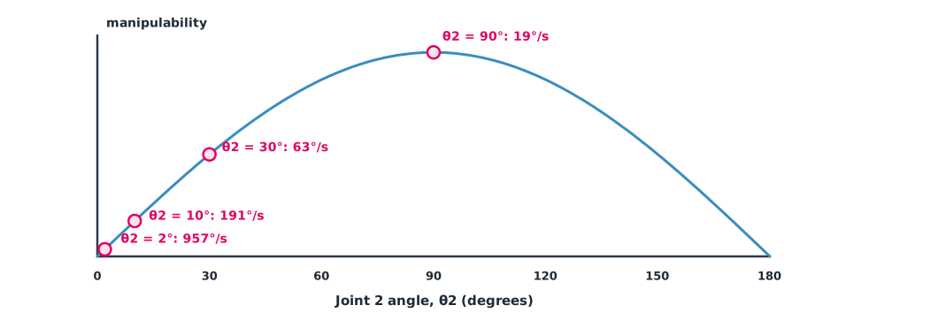
A two-joint arm with links of 0.40 and 0.30 m has its first joint at 0°. The tool must move outward along x at 0.10 m/s to push a battery into its slot. Compare different second-joint angles (simulated data).
import numpy as np

l1, l2 = 0.40, 0.30          # link lengths m
v_tool = np.array([0.10, 0.0])  # tool must move at 0.10 m/s

def jacobian(t1, t2):
    return np.array([
        [-l1*np.sin(t1) - l2*np.sin(t1+t2), -l2*np.sin(t1+t2)],
        [ l1*np.cos(t1) + l2*np.cos(t1+t2),  l2*np.cos(t1+t2)]])

t1 = np.radians(0)
for deg in [90, 30, 10, 2]:
    J = jacobian(t1, np.radians(deg))
    w = abs(np.linalg.det(J))
    qdot = np.linalg.solve(J, v_tool)
    print(f"θ2={deg:>2}°  manipulability={w:.4f}  "
          f"max joint speed={np.degrees(np.abs(qdot)).max():6.1f} deg/s")
θ2=90° manipulability=0.1200 max joint speed= 19.1 deg/s
θ2=30° manipulability=0.0600 max joint speed= 63.0 deg/s
θ2=10° manipulability=0.0208 max joint speed= 191.2 deg/s
θ2= 2° manipulability=0.0042 max joint speed= 957.4 deg/sThe straighter the arm (θ2 approaching 0), the lower the manipulability and the higher the joint speed needed, until it exceeds what typical motors can do. Working poses should therefore keep the arm reasonably bent, and the controller should limit joint speeds rather than try to follow impossible commands.
Numerical IK with damped least squares
With no closed form, inverse kinematics is solved iteratively. Each iteration computes the error between the target and the current tool position, then moves the joints by a obtained from the Jacobian. The pseudoinverse method () converges fast when the target is reachable, but near singularities it commands huge joint jumps. Buss (2004) explains the damped least squares (DLS) method, which adds to trade a little accuracy for smooth motion.
Example 2 A three-joint arm, a reachable target and one too far away
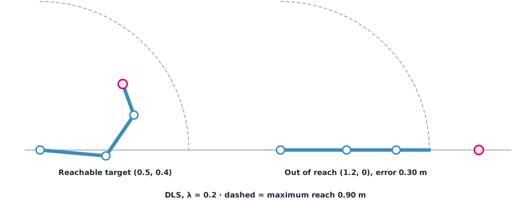
A three-joint arm has links of 0.40, 0.30 and 0.20 m (maximum reach 0.90 m). The first target is the battery slot at (0.50, 0.40) m; the second is a point out of reach at (1.20, 0) m. Compare λ = 0 with λ = 0.2 over 200 iterations (simulated data).
import numpy as np

L = np.array([0.40, 0.30, 0.20])     # three links, maximum reach 0.90 m

def fk(q):
    a = np.cumsum(q)
    return np.array([np.sum(L*np.cos(a)), np.sum(L*np.sin(a))])

def jac(q):
    a = np.cumsum(q)
    J = np.zeros((2, 3))
    for i in range(3):
        J[0, i] = -np.sum(L[i:]*np.sin(a[i:]))
        J[1, i] = np.sum(L[i:]*np.cos(a[i:]))
    return J

def ik(target, lam, iters=200):
    q = np.radians([10.0, 20.0, 20.0])
    max_step = 0.0
    for _ in range(iters):
        e = target - fk(q)
        J = jac(q)
        dq = J.T @ np.linalg.solve(J @ J.T + (lam**2 + 1e-12) * np.eye(2), e)
        max_step = max(max_step, np.degrees(np.abs(dq)).max())
        q = q + dq
    return np.linalg.norm(target - fk(q)), max_step

for lam in [0.0, 0.2]:
    for target in [np.array([0.50, 0.40]), np.array([1.20, 0.0])]:
        err, step = ik(target, lam)
        print(f"lambda={lam}  target {target}  error {err*1000:5.1f} mm  "
              f"largest joint step {step:6.1f} deg")
lambda=0.0 target [0.5 0.4] error 0.0 mm largest joint step 76.2 deg
lambda=0.0 target [1.2 0. ] error 799.9 mm largest joint step 1480.9 deg
lambda=0.2 target [0.5 0.4] error 0.0 mm largest joint step 22.7 deg
lambda=0.2 target [1.2 0. ] error 300.0 mm largest joint step 28.4 degWhen the target is reachable, both methods get there, but DLS moves the joints far less per iteration. When the target is out of reach, the pseudoinverse commands joint jumps of more than a thousand degrees per iteration and ends 0.80 m from the target, while DLS smoothly stretches the arm towards it and ends 0.30 m away, exactly the real shortfall (). A real system should first check whether the target is in the workspace and raise a warning instead of trying on.
Arm safety
An arm working near people and drones needs defined limits on workspace, speed and force. ISO 10218 (2025 edition) sets safety requirements for industrial robots and their use in robot cells. Although the UGV arm is small, the same principles apply: an emergency stop, joint speed limits, software limits on motion range, and an immediate stop when a person or still-spinning propeller is detected in the area.
Module lab
Lab: the Jacobian and IK on a training arm
- Measure the training arm’s link lengths, write forward kinematics and the Jacobian, and check them against 5 measured poses
- Use Example 1 to compute the joint speeds needed in real working poses and compare with the servos’ maximum speed
- Write DLS IK following Example 2, command the arm to 5 mock battery-slot positions, and measure the error with a ruler
- Try different λ values and record accuracy against smoothness of motion
- Write the arm’s working limits and emergency-stop conditions
Common mistakes
Watch out
- Designing working poses near singularities, such as keeping the arm fully stretched
- Using the pseudoinverse without limiting step size
- Not checking that the target is in the workspace before running IK
- Setting λ too large, so the arm cannot reach targets that are reachable
- Having no software limits or emergency stop
Summary
- The Jacobian converts joint velocity into tool velocity and can be used in reverse
- Near singularities, manipulability approaches zero and joint speeds soar
- DLS makes numerical IK smooth and robust to unreachable targets
- Arms need working limits and safety measures following the principles of ISO 10218
Check your understanding
- A two-joint arm with links of 0.4 and 0.3 m at θ2 = 90° has what manipulability?
- What is a singularity?
- Why can a fully stretched arm not push its tool further out?
- What does λ in DLS trade against what?
- A three-joint arm with 0.9 m total length has a target 1.1 m away. About what error will DLS leave?
Answers
- A pose where the Jacobian loses rank, so the tool cannot move in some directions
- Outward along the arm is a direction the Jacobian cannot produce in that pose
- A little accuracy for smooth motion without jumps
- About m
Key formulas
| Tool velocity | |
| Manipulability | |
| Damped least squares |
Key references
- Lynch, K. M., & Park, F. C. (2017). Modern robotics: Mechanics, planning, and control. Cambridge University Press. link
- Yoshikawa, T. (1985). Manipulability of robotic mechanisms. The International Journal of Robotics Research, 4(2), 3–9. link
- Buss, S. R. (2004). Introduction to inverse kinematics with Jacobian transpose, pseudoinverse and damped least squares methods [Unpublished manuscript]. University of California, San Diego. link
- Corke, P. (2023). Robotics, vision and control: Fundamental algorithms in Python. Springer. link
- International Organization for Standardization. (2025). Robotics – Safety requirements – Part 1: Industrial robots (ISO 10218-1:2025). link
Further reading
Study the assigned knowledge units in advance, review media and take the module quiz
In class / field
Lab or field practice from worksheets with a safety checklist
Learning evidence: Checked worksheets and quiz results