Sensor fusion
UAT 322 Artificial Intelligence and Autonomous Unmanned Aircraft Systems Integration Laboratory
Lesson
By the end of this module you will be able to
- Explain the predict–update principle of the Kalman filter and why fusion beats any single sensor
- Write a one-dimensional Kalman filter fusing IMU and GNSS that rejects outliers with an innovation gate
- Read sensor settings and test ratios of PX4 EKF2 and ArduPilot EKF3
- Calculate the reprojection RMSE of a camera–IMU calibration and state what must be reported with it
Why this matters
An IMU measures acceleration hundreds of times a second, but integrating acceleration into position lets small errors accumulate until the position drifts far away. GNSS gives position without drift, but only a few times a second, with metre-level noise, and sometimes jumps wrongly when signals reflect off buildings. Sensor fusion combines the strengths of both, like walking through a dark room counting steps and touching the wall now and then to correct the count.
The Kalman filter
A Kalman filter estimates a state (such as position and velocity) together with its uncertainty. Following Welch and Bishop, it loops through two steps:
- Predict: use a motion model and the IMU to move the state forward; the uncertainty grows every time
- Update: when a measurement such as GNSS arrives, compute the innovation , the measurement minus the prediction, then move the state towards the measurement weighted by the Kalman gain . The more the measurement is trusted (small R), the larger
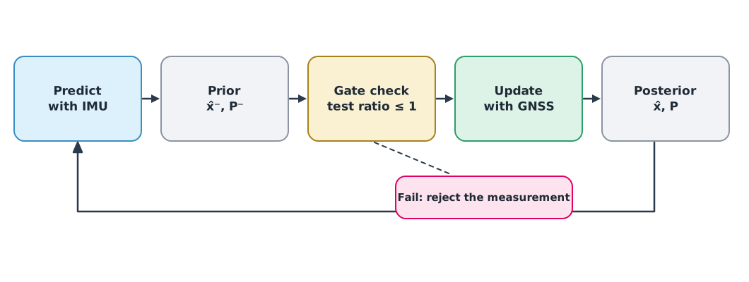
Before using a measurement, the system checks whether the innovation is larger than the uncertainty can explain, using the test ratio , where is the gate in standard deviations. Above 1, the measurement is rejected. PX4 EKF2 uses the same principle; its GNSS position gate (EKF2_GPS_P_GATE) defaults to 5 standard deviations.
Example 1 Fusing IMU and GNSS in one dimension
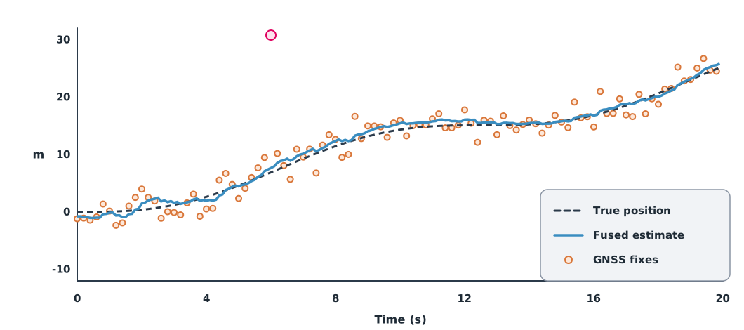
Twenty seconds of synthetic data: a 100 Hz IMU with a 0.05 m/s² bias and noise, and 5 Hz GNSS with 1.5 m noise and one +25 m error at 6 s.
import numpy as np

rng = np.random.default_rng(348)
dt = 0.01
t = np.arange(0, 20.0, dt)
true_acc = 0.6 * np.sin(0.5 * t)
true_pos = np.cumsum(np.cumsum(true_acc) * dt) * dt
imu_acc = true_acc + 0.05 + rng.normal(0, 0.2, t.size)
gnss = true_pos + rng.normal(0, 1.5, t.size)
gnss[600] += 25.0                                   # bad GNSS fix at t = 6 s

x, P = np.zeros(2), np.diag([4.0, 1.0])             # state [position, velocity]
F, B = np.array([[1, dt], [0, 1]]), np.array([0.5 * dt**2, dt])
Q, R, H, gate = np.diag([1e-4, 4e-4]), 1.5**2, np.array([1.0, 0.0]), 5.0
est, dead, vel, pos = np.zeros(t.size), np.zeros(t.size), 0.0, 0.0
for k in range(t.size):
    x, P = F @ x + B * imu_acc[k], F @ P @ F.T + Q          # predict
    vel += imu_acc[k] * dt
    pos += vel * dt
    dead[k] = pos                                             # IMU only
    if k % 20 == 0:                                           # GNSS every 0.2 s
        y = gnss[k] - H @ x
        S = H @ P @ H + R
        ratio = y**2 / (gate**2 * S)
        if ratio > 1:
            print(f"t = {t[k]:.1f} s: GNSS rejected, test ratio {ratio:.2f}")
        else:
            K = P @ H / S
            x, P = x + K * y, (np.eye(2) - np.outer(K, H)) @ P
    est[k] = x[0]
g = np.arange(0, t.size, 20)
rmse = lambda a, idx=slice(None): np.sqrt(np.mean((a[idx] - true_pos[idx]) ** 2))
print(f"RMSE  IMU only {rmse(dead):.2f} m | GNSS only {rmse(gnss, g):.2f} m | fused {rmse(est):.2f} m")
t = 6.0 s: GNSS rejected, test ratio 8.06
RMSE IMU only 4.82 m | GNSS only 2.94 m | fused 0.69 mThe bad GNSS fix has a test ratio of 8.06 and is rejected, so it does not drag the estimate with it. IMU alone errs by 4.82 m because the bias accumulates; GNSS alone by 2.94 m (including one 25 m error); the fused estimate by only 0.69 m. Q and R here were set for synthetic data whose answer is known; a real system must tune them from logs and sensor specifications.
The EKF in the flight controller
Real systems have dozens of states (position, velocity, attitude, sensor biases, magnetic field, wind) and nonlinear equations, so they use an Extended Kalman Filter (EKF) that linearises around the current estimate. Probabilistic Robotics explains the principle in detail.
- PX4 EKF2 fuses the IMU, magnetometer, GNSS, barometer, range finder, optical flow, external vision and airspeed; each source has its own test ratio, visible in the log
- ArduPilot EKF3 is ArduPilot’s default estimator
- Fusing position from a vision system (such as VIO) into EKF2 is enabled with
EKF2_EV_CTRL, a bitmask selecting horizontal position, vertical position, velocity or yaw; it is off by default
VIO (visual-inertial odometry), such as VINS-Mono and OpenVINS, estimates motion from a camera and an IMU and can replace GNSS indoors, but the camera and IMU must be calibrated well first.
Calibrating camera and IMU
Calibration has three parts: intrinsics (the camera model, such as focal length and distortion), extrinsics (the rotation and translation between camera and IMU) and time offset (the timing difference between the two sensors). Tools such as Kalibr report quality as reprojection error: the distance on the image between detected points and points projected from the model.
residuals = [(3, 4), (-1, 2), (0, -2), (2, 1)]      # (dx, dy) in pixels
n = len(residuals)
sq = sum(dx * dx + dy * dy for dx, dy in residuals)
print(f"RMSE per point {(sq / n) ** 0.5:.2f} px, per component {(sq / (2 * n)) ** 0.5:.2f} px")
RMSE per point 3.12 px, per component 2.21 pxThe same residuals give different numbers depending on the definition; OpenCV’s calibrateCamera divides by the number of points, so always state the definition. A small value on the calibration set does not confirm quality on new images; check with a separate data set, and record image resolution, lens, distortion model and target size with it.
Module lab
Lab: reading the EKF from logs and calibrating a camera
- Change
Randgatein Example 1 one at a time, recording the effect on RMSE and on rejected fixes. - Hover in SITL, open the log, and plot the test ratios of GNSS, barometer and magnetometer, identifying periods where they approach 1.
- Simulate GNSS loss in SITL and observe how EKF2 reports its status and how the drone changes mode.
- Photograph a calibration target with the onboard camera, calibrate with OpenCV or Kalibr, report reprojection RMSE with its definition, and check with a new image set.
- Record software versions, settings and all results in the lab notebook.
Common mistakes
Watch out
- Trusting every GNSS fix with no gate to reject outliers
- Setting R smaller than reality, so the filter chases noise
- Widening the gate so nothing is rejected, letting bad data in
- Enabling external vision without checking frames and timing
- Reporting reprojection error without its definition, or without checking on new data
Summary
- The Kalman filter predicts with a model and the IMU, then updates with measurements weighted by uncertainty
- An innovation gate uses the test ratio to reject outliers; above 1 is rejected
- PX4 EKF2 and ArduPilot EKF3 fuse many sources and log their test ratios
- Camera–IMU calibration covers intrinsics, extrinsics and time offset, and RMSE must be reported with its definition
Check your understanding
- Why does integrating IMU acceleration alone make position drift?
- Innovation m, m², gate . What is the test ratio, and is the measurement used?
- If R (measurement variance) increases, does the Kalman gain rise or fall?
- Two residuals are (3, 4) and (0, 0) px. What is the reprojection RMSE per point?
- Which PX4 parameter enables fusing position from a vision system?
Answers
- Small errors and biases are integrated twice, so they grow over time
- , so it is rejected
- It falls, because the measurement is trusted less
- px
EKF2_EV_CTRL
Key formulas
| Predict | |
| Update with a measurement | |
| Innovation test ratio | |
| Reprojection RMSE per point |
Key references
- Welch, G., & Bishop, G. (2004). An introduction to the Kalman filter (Tech. Rep. TR 95-041). Department of Computer Science, University of North Carolina at Chapel Hill. link
- Thrun, S., Burgard, W., & Fox, D. (2005). Probabilistic robotics. MIT Press. link
- PX4 Autopilot. Using the ECL EKF. PX4 user guide (main). link
- ArduPilot Dev Team. Extended Kalman filter (EKF) overview. ArduPilot Copter documentation. link
- Qin, T., Li, P., & Shen, S. (2018). VINS-Mono: A robust and versatile monocular visual-inertial state estimator. IEEE Transactions on Robotics, 34(4), 1004–1020. link
- Geneva, P., Eckenhoff, K., Lee, W., Yang, Y., & Huang, G. (2020). OpenVINS: A research platform for visual-inertial estimation. In 2020 IEEE International Conference on Robotics and Automation (pp. 4666–4672). link
Further reading
Study the assigned knowledge units in advance, review media and take the module quiz
State estimation with Kalman filters/EKF
Calibrating cameras and IMUs
How VIN, VIO and SLAM differ
In class / field
Intensive lab and field practice recorded in a lab notebook
Learning evidence: Lab notebook signed by the instructor