Obstacle avoidance and mapping
UAT 322 Artificial Intelligence and Autonomous Unmanned Aircraft Systems Integration Laboratory
Lesson
By the end of this module you will be able to
- Build an occupancy grid, inflate obstacles for aircraft size, and find a path with A*
- Calculate stopping distance with latency and compare it with sensor range
- Explain PX4 Collision Prevention and ArduPilot BendyRuler, with their limits
- Explain the principle of SLAM and evaluate a trajectory with ATE RMSE
Why this matters
An autonomous survey drone must answer three questions all the time: what is ahead, which way to go, and whether it can stop in time if something appears suddenly. Get any one wrong and the drone may hit a tree or a wall. This module practises the basic tools for all three questions, and how to measure how far the map and position the system builds can be trusted.
Occupancy grids and A*
An occupancy grid divides space into cells, each marked free or occupied. Proposed by Elfes (1989), the idea is still widely used because it merges data from many sensors into one table easily.
A drone is not a point, so obstacles must be inflated by the aircraft’s radius plus a safety margin before searching for a path. A* (Hart, Nilsson and Raphael, 1968) finds the shortest path by expanding the cell with the lowest , where is the cost so far and an estimate of the remaining distance. If never overestimates the true distance, A* is guaranteed to find the shortest path.
Example 1 Finding a path with A*
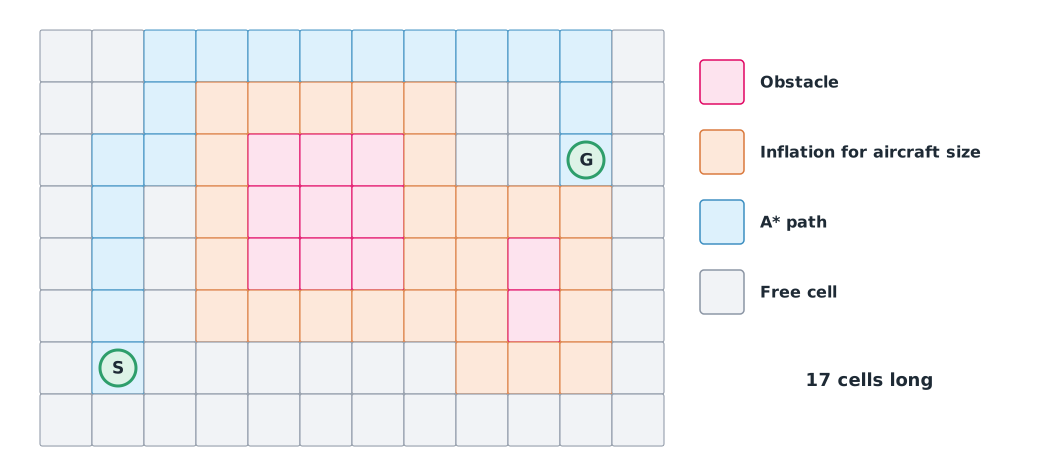
Each cell is 1 m wide, obstacles are inflated by 1 cell, and movement is in four directions.
import heapq

grid = ["............",
        "............",
        "....###.....",
        "....###.....",
        "....###..#..",
        ".........#..",
        "............",
        "............"]
ROWS, COLS = len(grid), len(grid[0])
start, goal = (6, 1), (2, 10)


def inflate(g, r=1):
    occ = {(i, j) for i in range(ROWS) for j in range(COLS) if g[i][j] == "#"}
    return {(i + a, j + b) for i, j in occ for a in range(-r, r + 1) for b in range(-r, r + 1)
            if 0 <= i + a < ROWS and 0 <= j + b < COLS}


def astar(blocked, s, g):
    h = lambda p: abs(p[0] - g[0]) + abs(p[1] - g[1])       # Manhattan distance never overestimates
    heap, came, cost, expanded = [(h(s), 0, s)], {s: None}, {s: 0}, 0
    while heap:
        _, c, p = heapq.heappop(heap)
        expanded += 1
        if p == g:
            break
        for d in ((1, 0), (-1, 0), (0, 1), (0, -1)):
            q = (p[0] + d[0], p[1] + d[1])
            if 0 <= q[0] < ROWS and 0 <= q[1] < COLS and q not in blocked and c + 1 < cost.get(q, 1e9):
                cost[q], came[q] = c + 1, p
                heapq.heappush(heap, (c + 1 + h(q), c + 1, q))
    path = [g]
    while came[path[-1]] is not None:
        path.append(came[path[-1]])
    return path[::-1], expanded


blocked = inflate(grid)
path, expanded = astar(blocked, start, goal)
print(f"path length {len(path) - 1} m, cells expanded {expanded}")
for i in range(ROWS):
    print("".join("S" if (i, j) == start else "G" if (i, j) == goal else "*" if (i, j) in path
                  else "#" if grid[i][j] == "#" else "+" if (i, j) in blocked else "." for j in range(COLS)))
path length 17 m, cells expanded 56
..*********.
..*+++++..*.
.**+###+..G.
.*.+###++++.
.*.+###++#+.
.*.++++++#+.
.S......+++.
............# marks obstacles, + the inflation and * the path. A* avoids both obstacles and inflation. The path follows the grid in right angles, so real systems smooth it before sending it as setpoints.
Can it stop in time?
Stopping distance has two parts: the distance travelled during the latency before braking starts, and the braking distance, just as a driver must count the time before the foot reaches the brake pedal.
v, latency, decel, sensor_range = 5.0, 0.25, 3.0, 8.0   # m/s, s, m/s², m
reaction = v * latency
braking = v ** 2 / (2 * decel)
stop = reaction + braking
print(f"reaction {reaction:.2f} m + braking {braking:.2f} m = {stop:.2f} m (sensor range {sensor_range} m)")
v_max = (-latency + (latency**2 + 2 * sensor_range / decel) ** 0.5) * decel
print(f"highest speed that still stops within the sensor range: {v_max:.2f} m/s")
reaction 1.25 m + braking 4.17 m = 5.42 m (sensor range 8.0 m)
highest speed that still stops within the sensor range: 6.22 m/s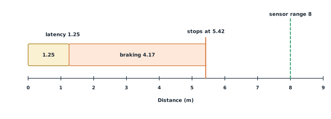
At 5 m/s the drone stops within 5.42 m, less than the 8 m sensor range, but the highest speed that still stops in time is only about 6.2 m/s. In practice, allow more for wind, position error and objects the sensor may miss, such as power lines.
Avoidance in the flight controller
- PX4 Collision Prevention works only in multicopter Position mode. It limits speed near obstacles, using distance data from a range sensor or from the companion computer via the
OBSTACLE_DISTANCEmessage. The distance to keep is set withCP_DIST, whose default of −1 means disabled - ArduPilot offers several levels, from Simple avoidance that stops in front of obstacles, to BendyRuler, which finds a way around them (in Auto, Guided and RTL modes), and Dijkstra’s, which plans around known fences and exclusion zones
These systems depend entirely on sensors: if the sensor cannot see an object, the system cannot avoid it. They are an extra layer of protection, not a reason to fly close to obstacles.
SLAM and trajectory evaluation
SLAM (simultaneous localization and mapping) builds a map and locates the vehicle in it at the same time, for places without GNSS such as indoors or under bridges. Cadena et al. (2016) review the development of SLAM, and ORB-SLAM3 is an open library supporting monocular, stereo and visual–inertial set-ups.
A common quality measure is the absolute trajectory error (ATE) from the benchmark of Sturm et al. (2012): the RMSE of the distance between estimated and true positions. Zhang and Scaramuzza (2018) warn that the two trajectories must first be aligned in a common frame, and the alignment method must always be stated.
import numpy as np

truth = np.array([[0, 0], [1, 0], [2, 0], [3, 0], [4, 0], [5, 0]], dtype=float)
estimate = np.array([[0, 0], [1.1, 0.1], [2.1, 0.2], [3.2, 0.2], [4.2, 0.3], [5.3, 0.4]])
errors = np.linalg.norm(estimate - truth, axis=1)
print("error per pose (m):", np.round(errors, 2))
print(f"ATE RMSE {np.sqrt(np.mean(errors ** 2)):.3f} m, final drift {errors[-1]:.2f} m")
error per pose (m): [0. 0.14 0.22 0.28 0.36 0.5 ]
ATE RMSE 0.297 m, final drift 0.50 mThe error grows with distance, the signature of drift. The two sets here already share a frame, so no alignment is needed; real data must be aligned first.
Module lab
Lab: obstacle avoidance in SITL
- Change the map in Example 1 to include a narrow gap, then try inflation of 0, 1 and 2 cells, recording when the path changes or cannot be found.
- Enable Collision Prevention in PX4 SITL with a simulated range sensor, set
CP_DIST, and fly towards a wall in Position mode, recording where the drone actually stops. - Vary speed and latency in the stopping-distance formula and compare with the SITL results.
- Using the trajectory data set prepared by the instructor, calculate ATE RMSE and explain the alignment used.
- Conclude the highest safe speed for the training drone’s sensor, with your assumptions.
Common mistakes
Watch out
- Not inflating obstacles for aircraft size, so paths graze obstacles and propellers strike
- Forgetting latency in stopping distance and counting only braking
- Assuming Collision Prevention is already on, when it is off by default
- Believing the sensor sees everything, although wires, glass and thin branches may be missed
- Reporting ATE without stating the alignment
Summary
- An occupancy grid represents space as cells; inflate obstacles for aircraft size before path finding
- A* expands the cell with the lowest and finds the shortest path when never overestimates
- Stopping distance is latency distance plus braking distance, and must be less than sensor range with a margin
- PX4 and ArduPilot have built-in avoidance, but it depends on sensors and must be enabled
- SLAM builds a map and localises at once, and is evaluated with ATE after alignment
Check your understanding
- In A*, if and , what is for that cell?
- At 4 m/s with 0.5 s latency and 2 m/s² braking, what is the stopping distance?
- Why must obstacles be inflated before path finding?
- What does the PX4 default
CP_DIST = −1mean? - Position errors at three poses are 0, 3 and 4 m. What is the ATE RMSE?
Answers
- m
- The drone has size; its centre must stay at least its radius plus a margin from obstacles
- Collision Prevention is disabled
- m
Key formulas
| A* cost | |
| Stopping distance | |
| ATE RMSE |
Key references
- Elfes, A. (1989). Using occupancy grids for mobile robot perception and navigation. Computer, 22(6), 46–57. link
- Hart, P. E., Nilsson, N. J., & Raphael, B. (1968). A formal basis for the heuristic determination of minimum cost paths. IEEE Transactions on Systems Science and Cybernetics, 4(2), 100–107. link
- PX4 Autopilot. Collision prevention. PX4 user guide (main). link
- ArduPilot Dev Team. Object avoidance. ArduPilot Copter documentation. link
- Cadena, C., Carlone, L., Carrillo, H., Latif, Y., Scaramuzza, D., Neira, J., Reid, I., & Leonard, J. J. (2016). Past, present, and future of simultaneous localization and mapping: Toward the robust-perception age. IEEE Transactions on Robotics, 32(6), 1309–1332. link
- Campos, C., Elvira, R., Gómez Rodríguez, J. J., Montiel, J. M. M., & Tardós, J. D. (2021). ORB-SLAM3: An accurate open-source library for visual, visual–inertial, and multimap SLAM. IEEE Transactions on Robotics, 37(6), 1874–1890. link
- Sturm, J., Engelhard, N., Endres, F., Burgard, W., & Cremers, D. (2012). A benchmark for the evaluation of RGB-D SLAM systems. In 2012 IEEE/RSJ International Conference on Intelligent Robots and Systems (pp. 573–580). link
- Zhang, Z., & Scaramuzza, D. (2018). A tutorial on quantitative trajectory evaluation for visual(-inertial) odometry. In 2018 IEEE/RSJ International Conference on Intelligent Robots and Systems (pp. 7244–7251). link
Further reading
Study the assigned knowledge units in advance, review media and take the module quiz
Autonomous path planning and obstacle avoidance
SLAM and GNSS-denied navigation
Exercise: measuring trajectory error
LiDAR, radar and obstacle-avoidance sensors
In class / field
Intensive lab and field practice recorded in a lab notebook
Learning evidence: Lab notebook signed by the instructor